A torchtensor is a multidimensional grid of values, all of the same type, and is indexed by a tuple of nonnegative integers. The number of dimensions is the rank of the tensor; the shape of a tensor is a tuple of integers giving the size of the array along each dimension.
We can initialize torch tensor from nested Python lists. We can access or mutate elements of a PyTorch tensor using square brackets.
Accessing an element from a PyTorch tensor returns a PyTorch scalar; we can convert this to a Python scalar using the .item() method
Tensor constructors
PyTorch provides many convenience methods for constructing tensors; this avoids the need to use Python lists, which can be inefficient when manipulating large amounts of data. Some of the most commonly used tensor constructors are:
torch.rand: Creates a tensor with uniform random numbers
Datatypes
Each tensor has a dtype attribute that you can use to check its data type
We can cast a tensor to another datatype using the .to() method; there are also convenience methods like .float() and .long() that cast to particular datatypes
PyTorch provides several ways to create a tensor with the same datatype as another tensor:
PyTorch provides tensor constructors such as torch.zeros_like() that create new tensors with the same shape and type as a given tensor
Tensor objects have instance methods such as .new_zeros() that create tensors the same type but possibly different shapes
The tensor instance method .to() can take a tensor as an argument, in which case it casts to the datatype of the argument
Tensor indexing
Slice indexing
similar to python
There are two common ways to access a single row or column of a tensor: using an integer will reduce the rank by one, and using a length-one slice will keep the same rank.
you can use the clone() method to make a copy of a tensor
Integer tensor indexing
We can also use index arrays to index tensors
More generally, given index arrays idx0 and idx1 with N elements each, a[idx0, idx1] is equivalent to:
Boolean tensor indexing lets you pick out arbitrary elements of a tensor according to a boolean mask. Frequently this type of indexing is used to select or modify the elements of a tensor that satisfy some condition.
In PyTorch, we use tensors of dtype torch.bool to hold boolean masks
1 2 3 4 5 6 7 8 9 10 11 12 13 14 15 16 17
# Find the elements of a that are bigger than 3. The mask has the same shape as # a, where each element of mask tells whether the corresponding element of a # is greater than three. mask = (a > 3) print('\nMask tensor:') print(mask)
# We can use the mask to construct a rank-1 tensor containing the elements of a # that are selected by the mask print('\nSelecting elements with the mask:') print(a[mask])
# We can also use boolean masks to modify tensors; for example this sets all # elements <= 3 to zero: a[a <= 3] = 0 print('\nAfter modifying with a mask:') print(a)
Reshaping operations
View
PyTorch provides many ways to manipulate the shapes of tensors. The simplest example is .view(): This returns a new tensor with the same number of elements as its input, but with a different shape.
We can use .view() to flatten matrices into vectors, and to convert rank-1 vectors into rank-2 row or column matrices
As a convenience, calls to .view() may include a single -1 argument; this puts enough elements on that dimension so that the output has the same number of elements as the input.
shares the same data!
Swapping axes
The simplest such function is .t(), specificially for transposing matrices
For tensors with more than two dimensions, we can use the function torch.transpose) to swap arbitrary dimensions.
If you want to swap multiple axes at the same time, you can use torch.permute) method to arbitrarily permute dimensions
Contiguous tensors
you can typically overcome these sorts of errors by either by calling .contiguous() before .view(), or by using .reshape() instead of .view()
Tensor operations
Elementwise operations
Basic mathematical functions operate elementwise on tensors, and are available as operator overloads, as functions in the torch module, and as instance methods on torch objects
Reduction operations
We may sometimes want to perform operations that aggregate over part or all of a tensor, such as a summation; these are called reduction operations.
Like the elementwise operations above, most reduction operations are available both as functions in the torch module and as instance methods on tensor objects.
We can use the .sum() method (or eqivalently torch.sum) to reduce either an entire tensor, or to reduce along only one dimension of the tensor using the dim argument.Other useful reduction operations include mean, min, and max
After summing with dim=d, the dimension at index d of the input is eliminated from the shape of the output tensor
Reduction operations reduce the rank of tensors: the dimension over which you perform the reduction will be removed from the shape of the output. If you pass keepdim=True to a reduction operation, the specified dimension will not be removed; the output tensor will instead have a shape of 1 in that dimension
torch.argmin:This is the second value returned by torch.min()
torch.addmm / torch.addmv: Computes matrix-matrix and matrix-vector multiplications plus a bias
torch.bmm / torch.baddmm: Batched versions of torch.mm and torch.addmm, respectively
torch.matmul: General matrix product that performs different operations depending on the rank of the inputs. Confusingly, this is similar to np.dot in numpy
torch.stack(tensors, dim=0, **, out=None*) :Concatenates a sequence of tensors along a new dimension
Vectorization
avoiding explicit Python loops in your code and instead using PyTorch operators to handle looping internally will cause your code to run a lot faster. This style of writing code, called vectorization, avoids overhead from the Python interpreter, and can also better parallelize the computation (e.g. across CPU cores, on on GPUs)
Broadcasting
Broadcasting usually happens implicitly inside many PyTorch operators. However we can also broadcast explicitly using the function torch.broadcast_tensors
In-place operators: modify and return the input tensor
Running on GPU
ll PyTorch tensors also have a device attribute that specifies the device where the tensor is stored — either CPU, or CUDA (for NVIDA GPUs)
we can use the .to() method to change the device of a tensor. We can also use the convenience methods .cuda() and .cpu() methods to move tensors between CPU and GPU
Calling x.to(y) where y is a tensor will return a copy of x with the same device and dtype as y
Other
torch.topk(input, k, dim=None, largest=True, sorted=True, **, out=None*):Returns the k largest elements of the given input tensor along a given dimension
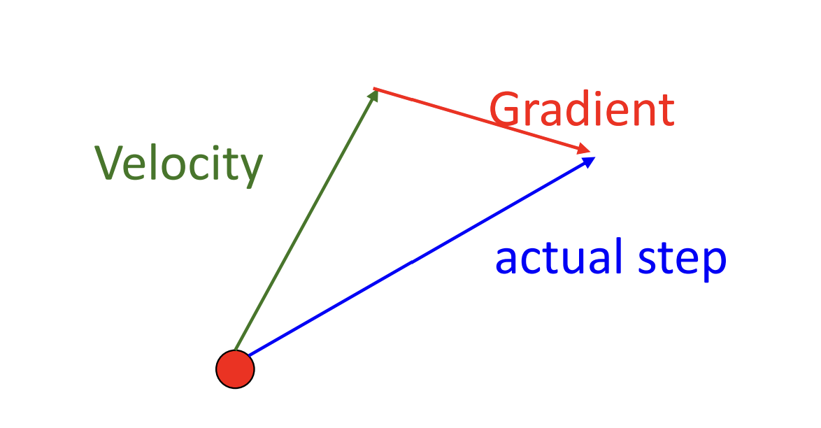
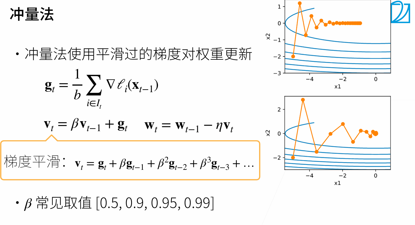
Build up “velocity” as a running mean of gradients
$\rho$ gives “friction”;typically rho=0.9 or 0.99
$v_{t+1}=\rho v_t+\nabla f(x_t)$
$x{t+1}=x_t-\alpha v{t+1}$
1).At local minimum we still have some velocity that can help escape
2).smooth out the noise ,alleviate oscillatory problem
Nesterov Momentum
“Look ahead” to the point where updating using velocity would take us; compute gradient there and mix it with velocity to get actual update direction
$v_{t+1}=\rho v_t-\alpha\nabla f(x_t+\rho v_t)$
$x{t+1}=x_t+v{t+1}$
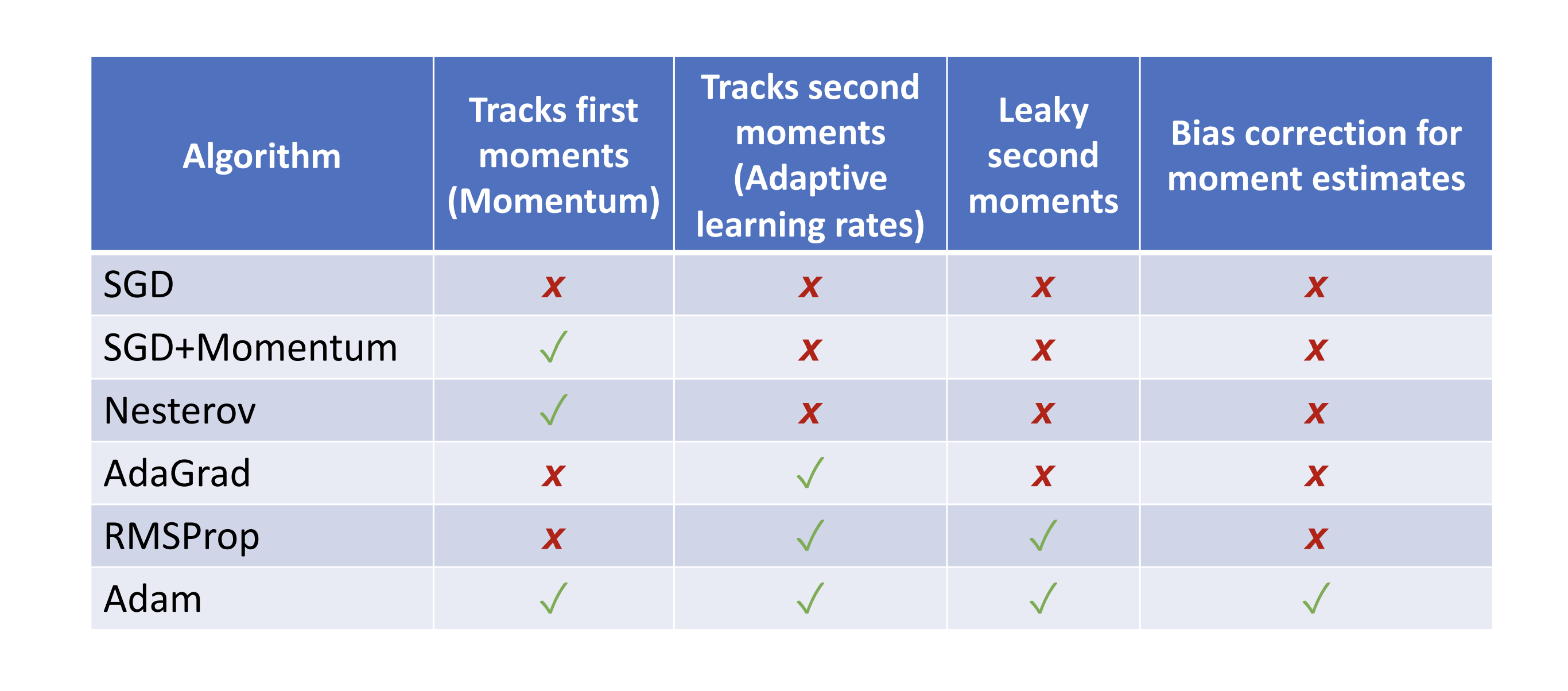
AdaGrad
1 2 3 4 5
grad_squared=0 for t inrange(num_steps): dw=compute_gradient(w) grad_squared+=dw*dw w-=learning_rate*dw/(grad_quared.sqrt()+1e-7)
progress along “steep”directions is damped
progress along “flat”directions is accelerated
RMSProp:”Leak Adagrad”
1 2 3 4 5
grad_squared=0 for t inrange(num_steps): dw=compute_gradient(w) grad_squared+=decay_rate*grad_squared+(1-decay_rate)*dw*dw w-=learning_rate*dw/(grad_quared.sqrt()+1e-7)
avoid slowing down when square becomes bigger
Adam: RMSProp+Momentum
1 2 3 4 5 6 7
moment1=0 moment2=0 for t inrange(num_steps): dw=compute_gradient(w) moment1=beta1*moment1+(1-beta1)*dw #similar to velocity moment2=beta2*moment2+(1-beta2)*dw*dw w-=learning_rate*moment1/(moment2.sqrt()+1e-7)
Bias correction for the fact that the first and the second moment estimates start at zero
1 2 3 4 5 6 7 8 9
moment1=0 moment2=0 for t inrange(num_steps): dw=compute_gradient(w) moment1=beta1*moment1+(1-beta1)*dw #similar to velocity moment2=beta2*moment2+(1-beta2)*dw*dw moment1_unbias=moment1/(1-beta1**t) moment2_unbias=moment2/(1-beta2**t) w-=learning_rate*moment1_unbias/(moment2_unbias.sqrt()+1e-7)
lecture 5:Neural Networks
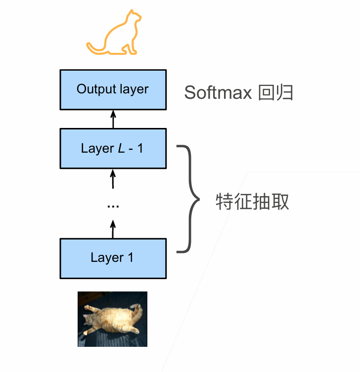
Feature transforms
Fully-connected neural network:also MLP
Lecture 6:Back Propagation
Represent complex expressions as computational graphs
During the backward pass, each node in the graph receives upstream gradients and multiplies them by local gradients to compute downstream gradients
Backprop can be implemented with “flat” code where the backward pass looks like forward pass reversed
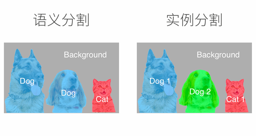
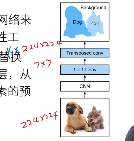
Lecture 7:Convolutional Networks
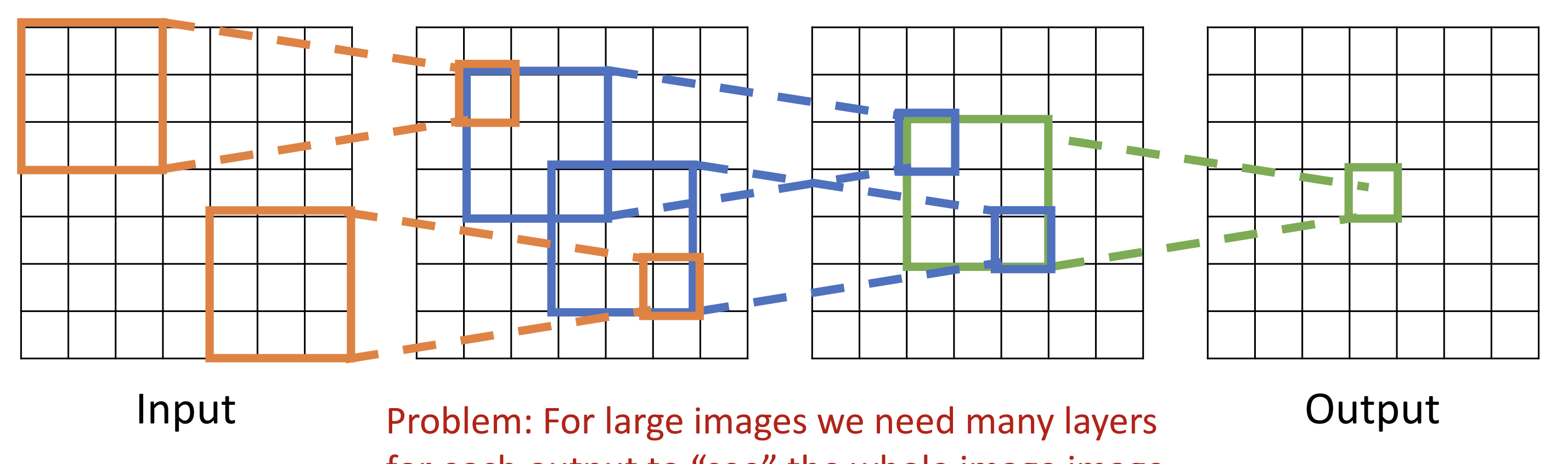
Receptive Fields
Each successive convolution adds K-1 to the receptive field size
With L layers the receptive field size is 1+L*(K-1)
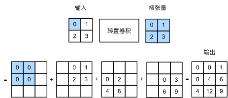
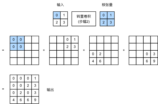
Strided Convolution
a way to add receptive field size quickly
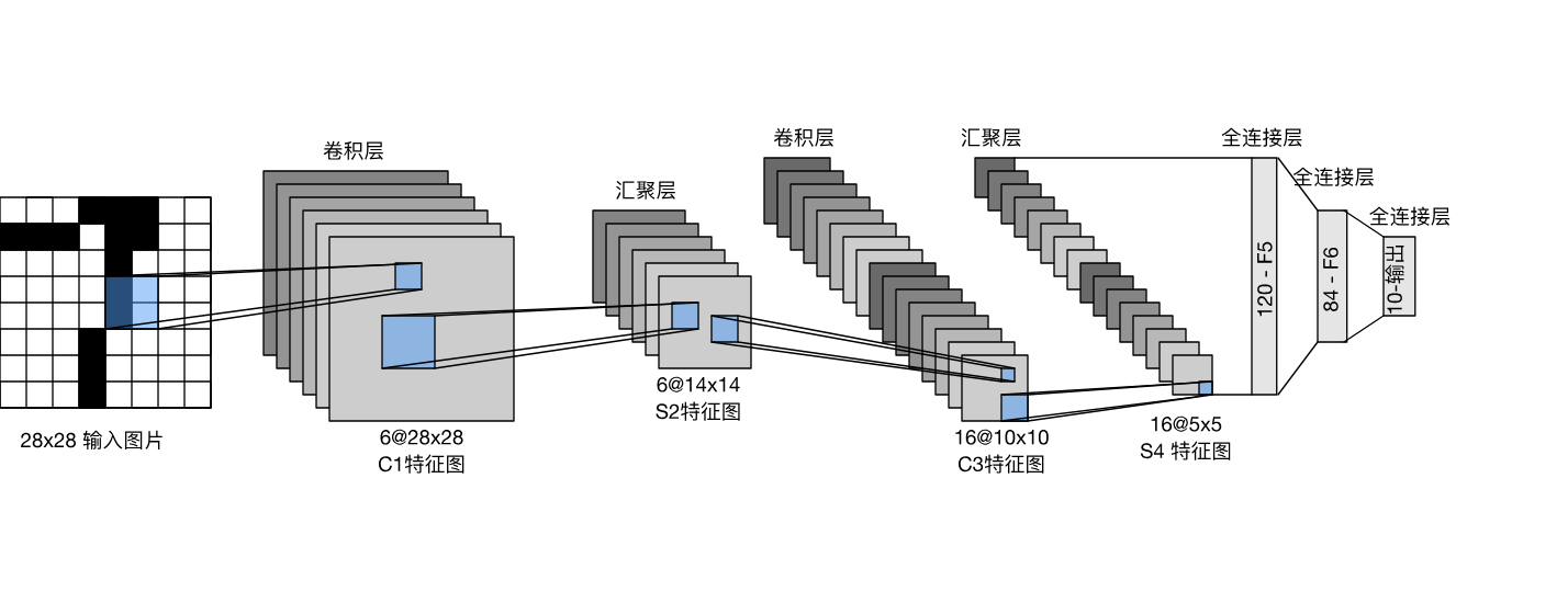
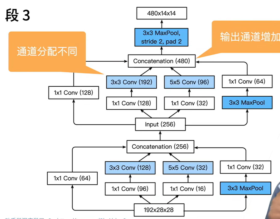
LeNet
spatial size decreases:using pooling or strived conv
number of channels increases:total “volume” is preserved
Lecture 8:CNN Architecture
ZFNet:a bigger AlexNet
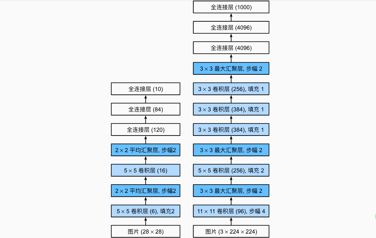
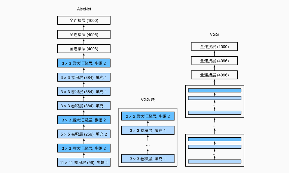
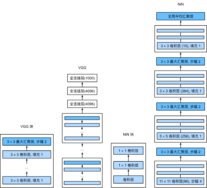
VGG
5x5=2 layer of 3x3 in receptive fields,but less FLOPS and fewer parametres;and it can add more relu between layers
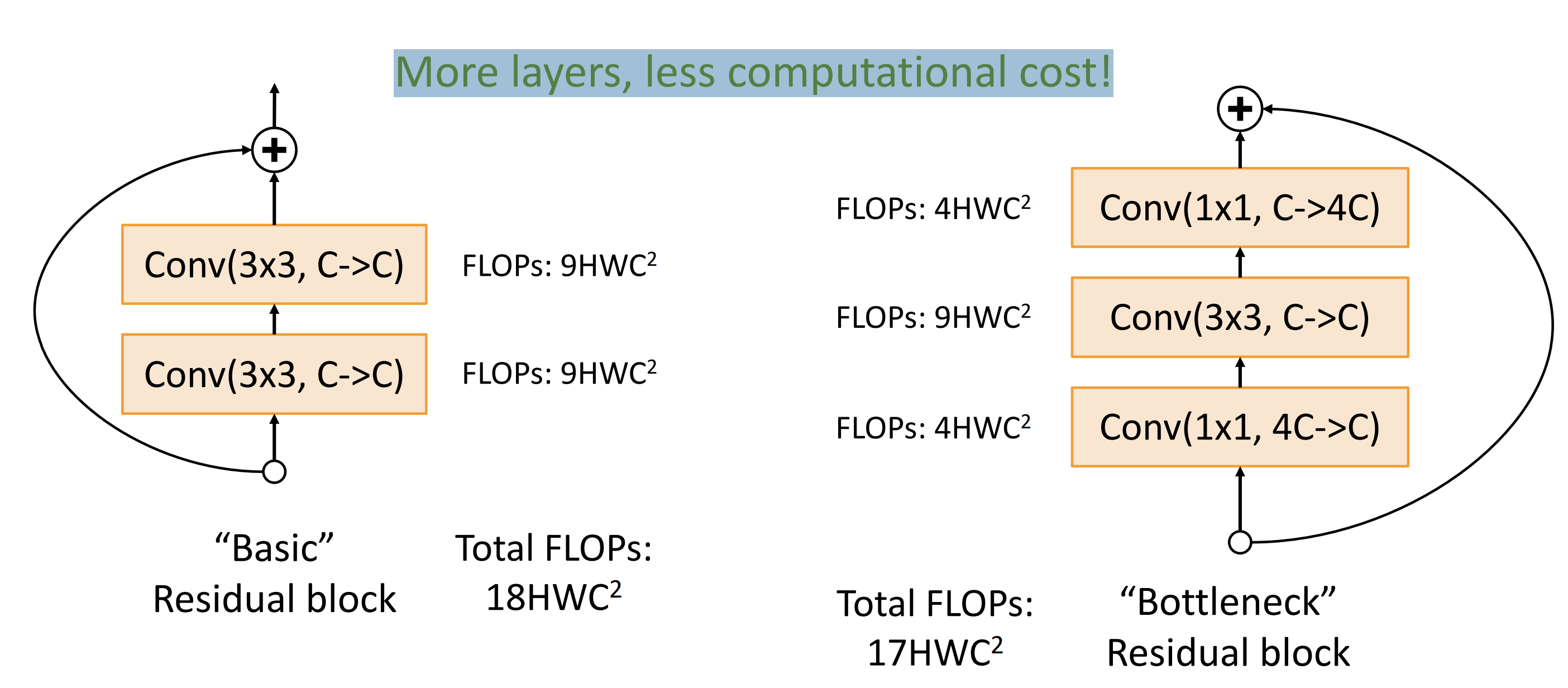
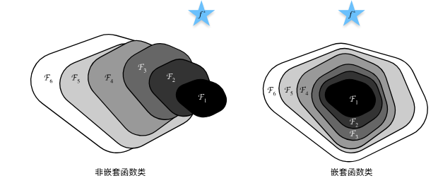
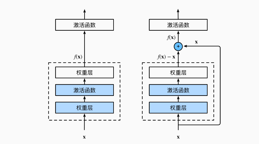
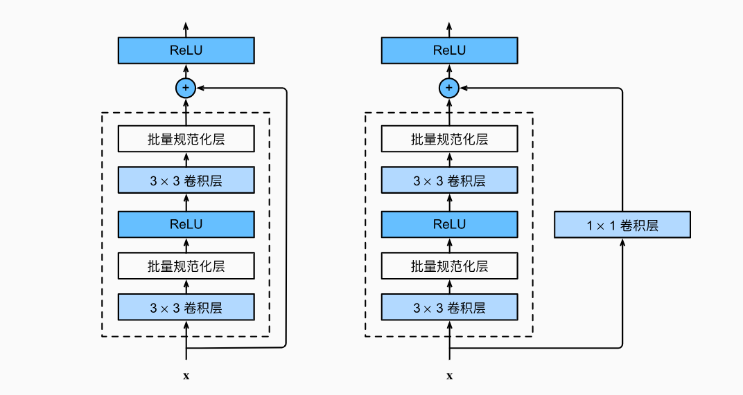
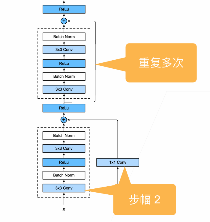
ResNet
Bottleneck Block:More layers, less computational cost
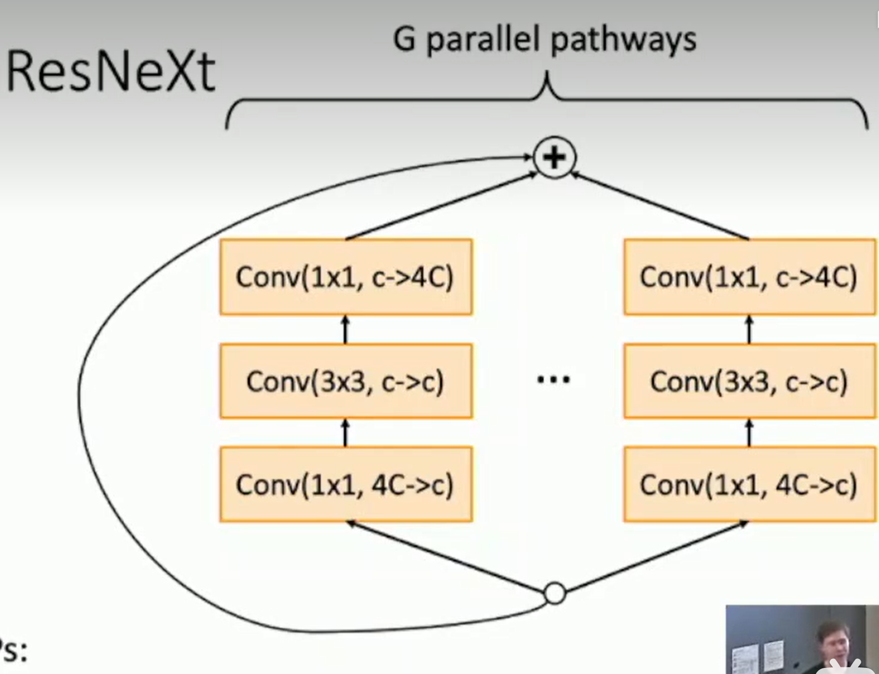
ResNeXt
add groups improves performance with same computational complexity
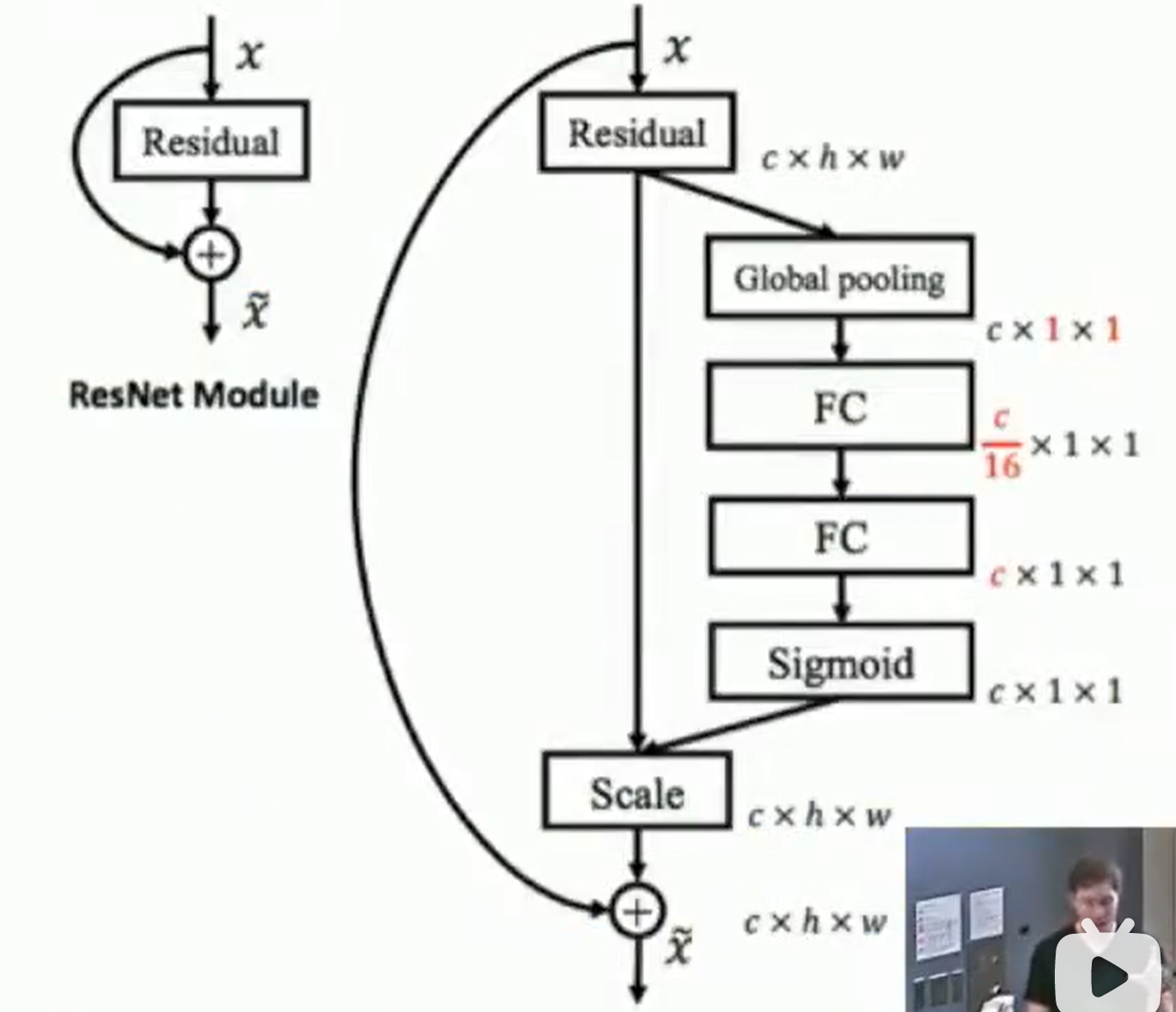
Squeeze-and-Excitation Networks
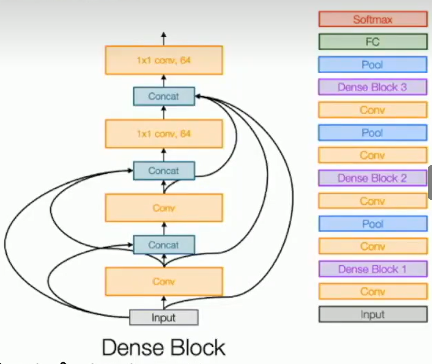
Densely Connected Neural Networks
Dense blocks where each layer is connected to every other layer in feedforward fashion
3.After training Model ensembles, transfer learning
Learning Rate Schedule
Learing Rate Decay:Step
reduce learning rate at a few fixed points
Learing Rate Decay:Sosine
$\alpha_t=1/2\alpha_0(1+cos(t\pi/T))$
Learing Rate Decay:Linear
$\alpha_t=\alpha_0(1-t/T)$
Learing Rate Decay:Inverse Sqrt
$\alpha_t=\alpha_0/\sqrt{t}$
Choosing Hyperparameters
grid search
random search
Model Ensembles
Train multiple independent models 2. At test time average their results
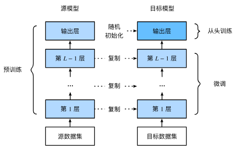
Transfer Learning
feature extracter;fine tuning
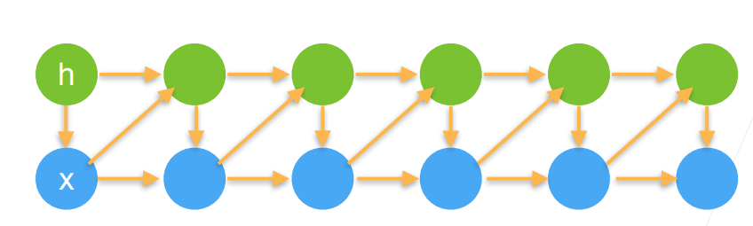
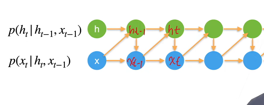
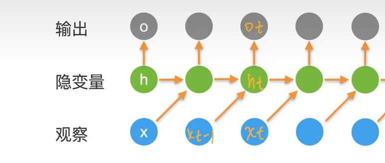
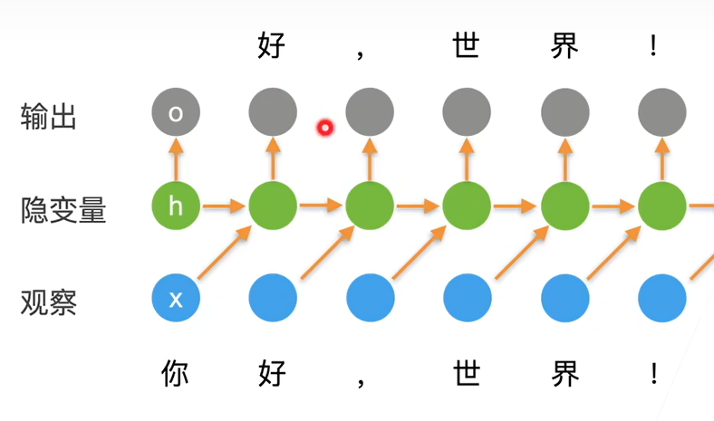
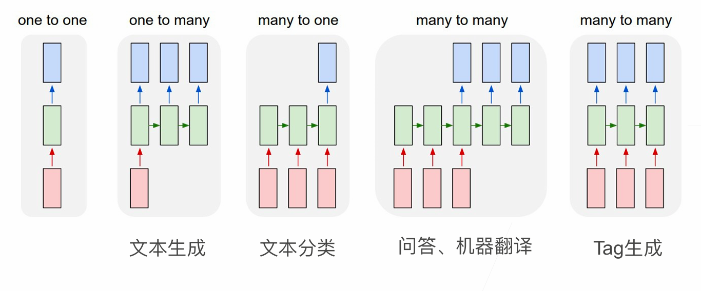
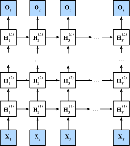
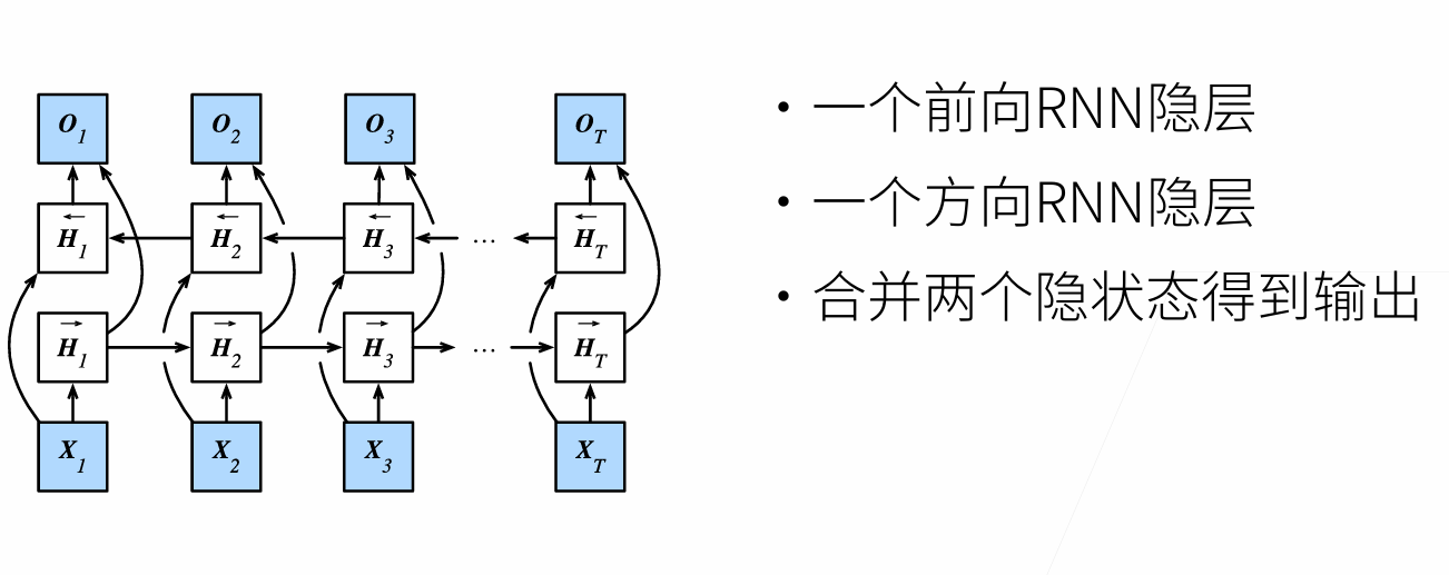
Lecture 12: Recurrent Networks
key idea: RNNs have an “internal state” that is updated as a sequence is processed
$ht=f_W(h{t-1},x_t)$
Vanilla/Elman RNN
$ht=tanh(W{hh}h{t-1}+W{xh}x_t)$
$y{t}=W{hy}h_{t}$
Truncated Backpropagation Through Time
only backpropagate through finite chunks of the sequence
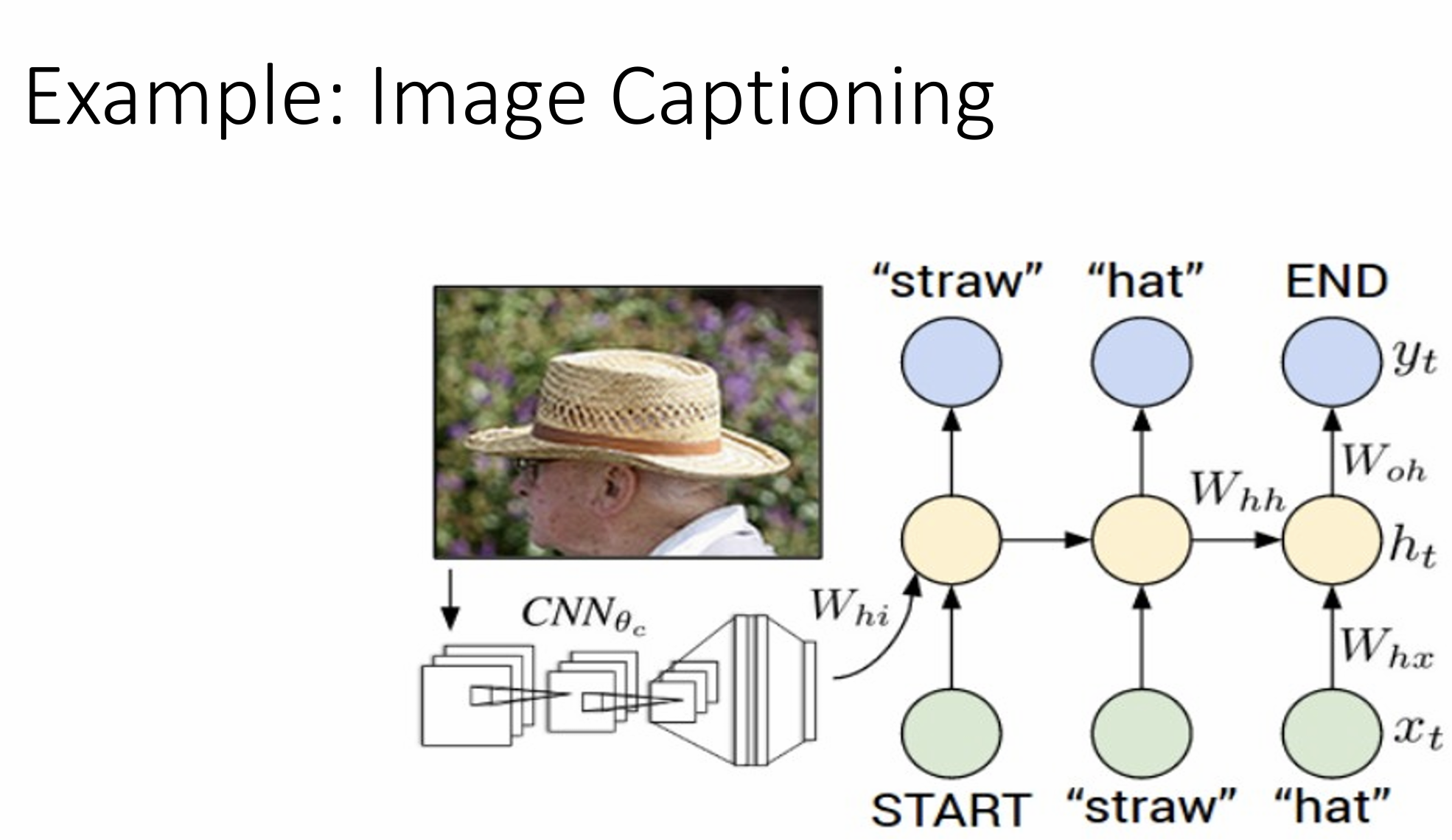
Example: Image Captioning
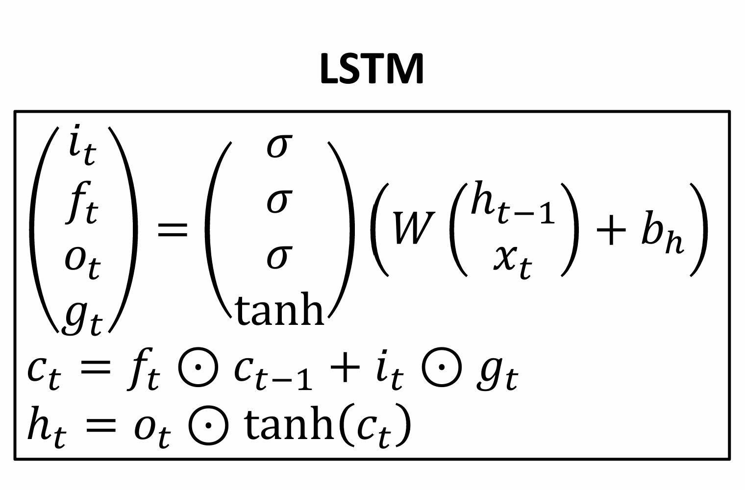
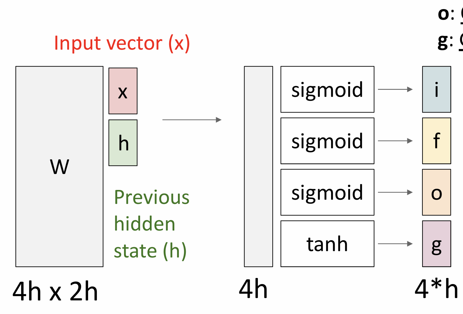
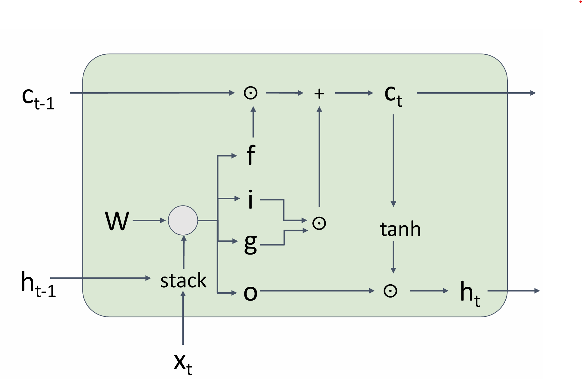
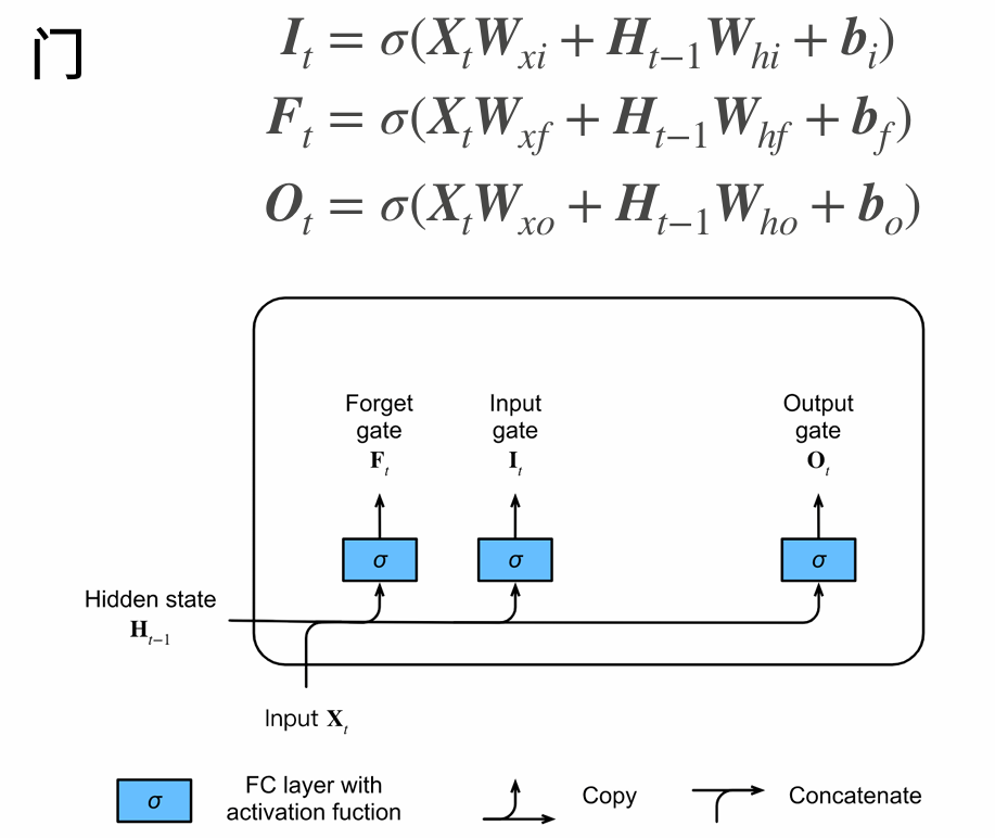
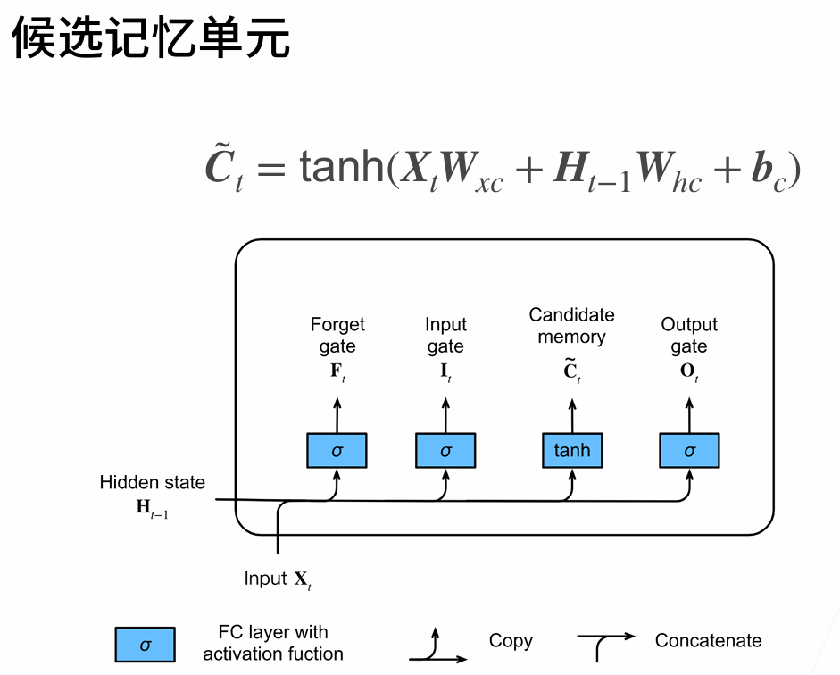
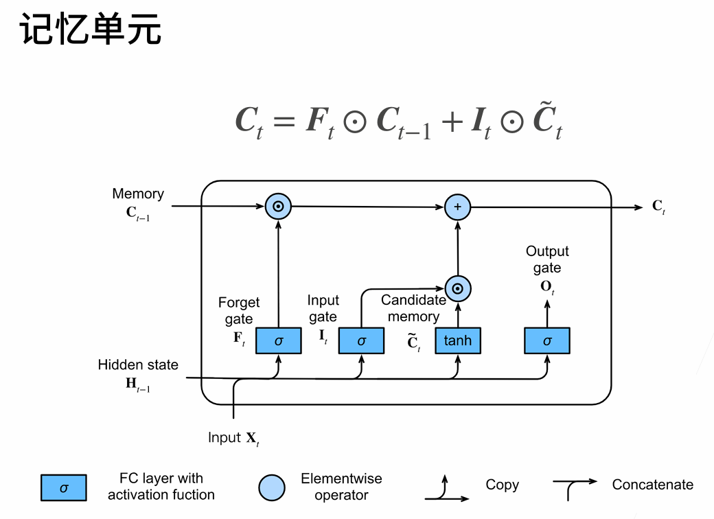
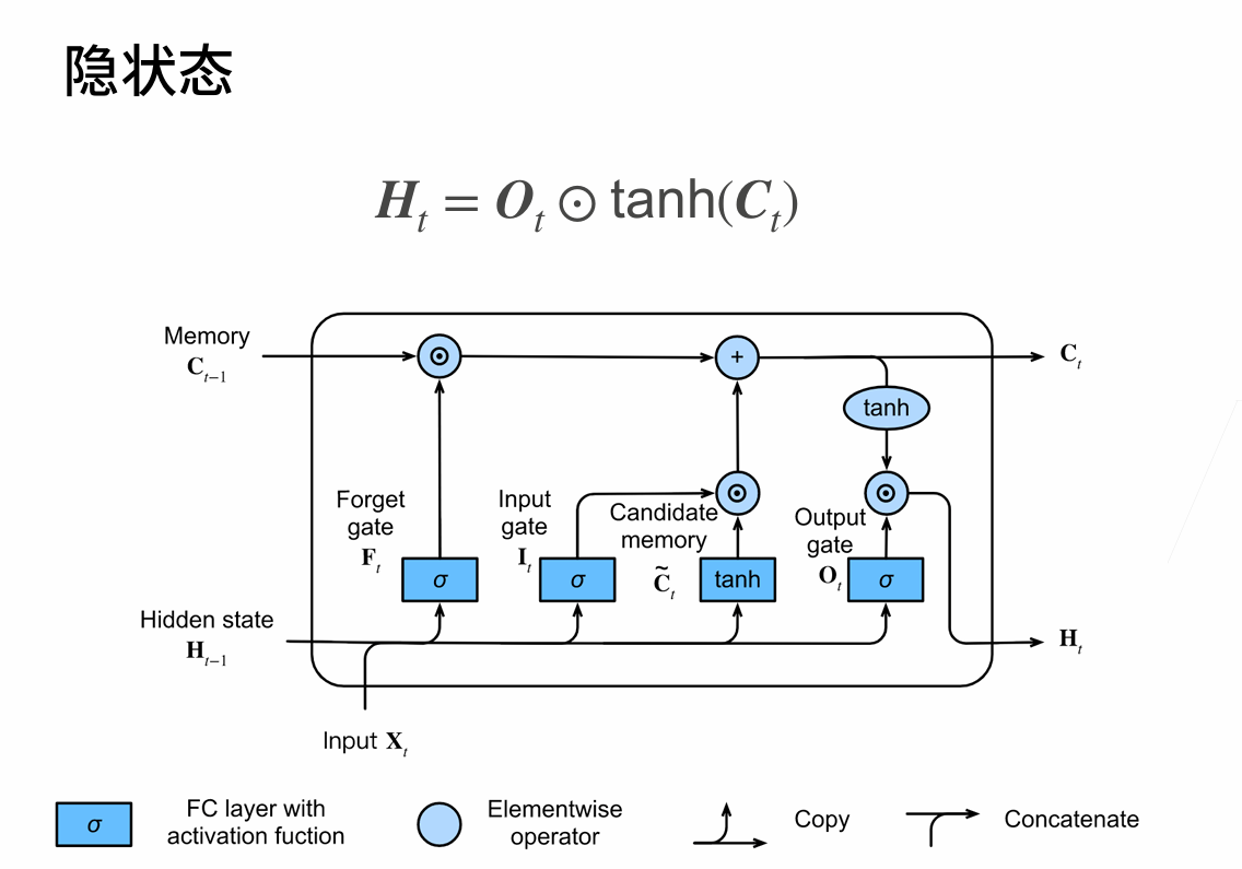
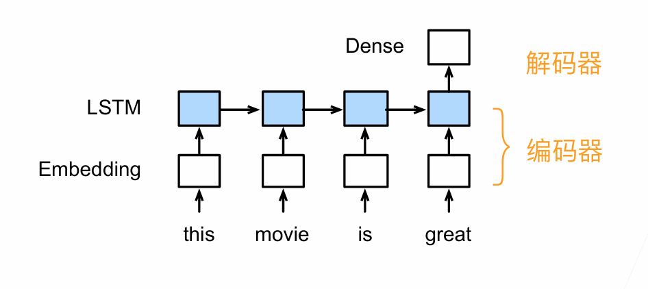
Long Short Term Memory(LSTM)
two vectors at each timestep: cell state and hidden state
four gates
i:input gate,whether to write cell
f: forget gate,whether to erase cell
o:output gate,whether to reveal cell
g:gategate,how much to write to cell
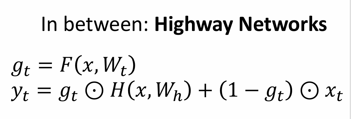
Highway Networks
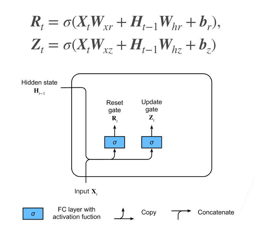
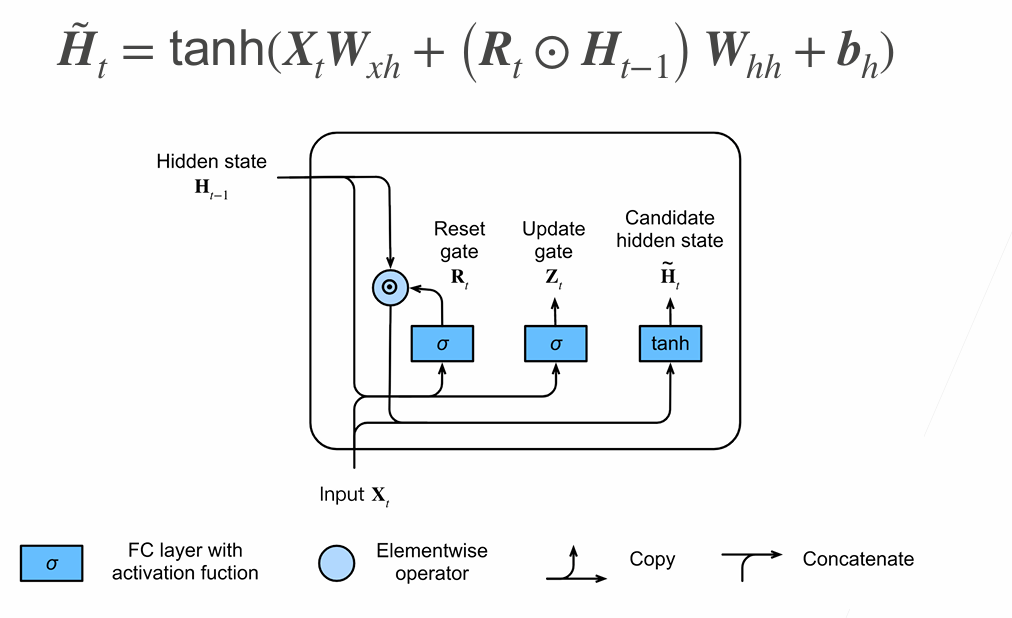
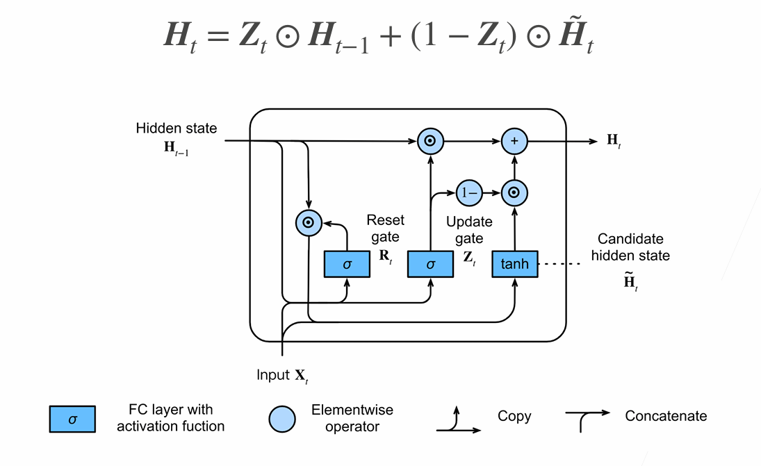
Gated Recurrent Unit(GRU)
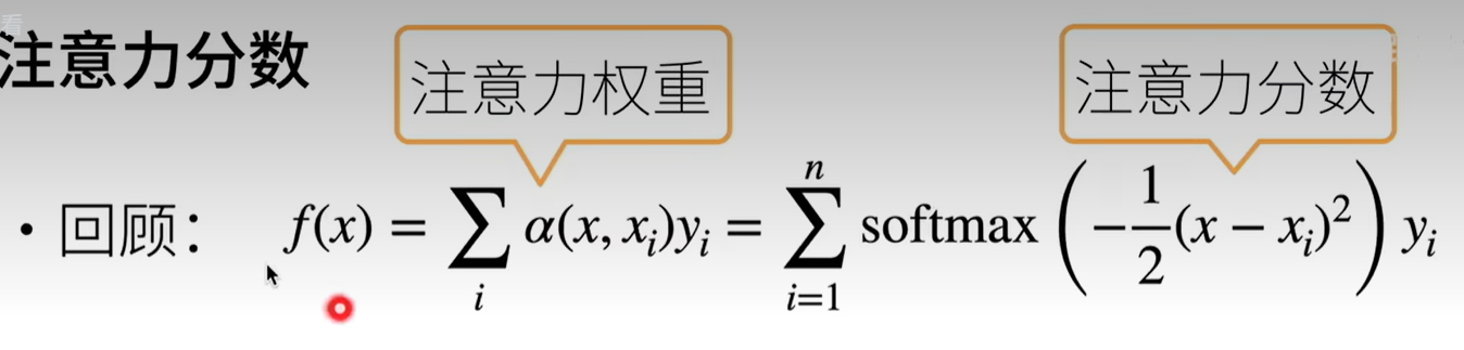
Lecture 13: Attention
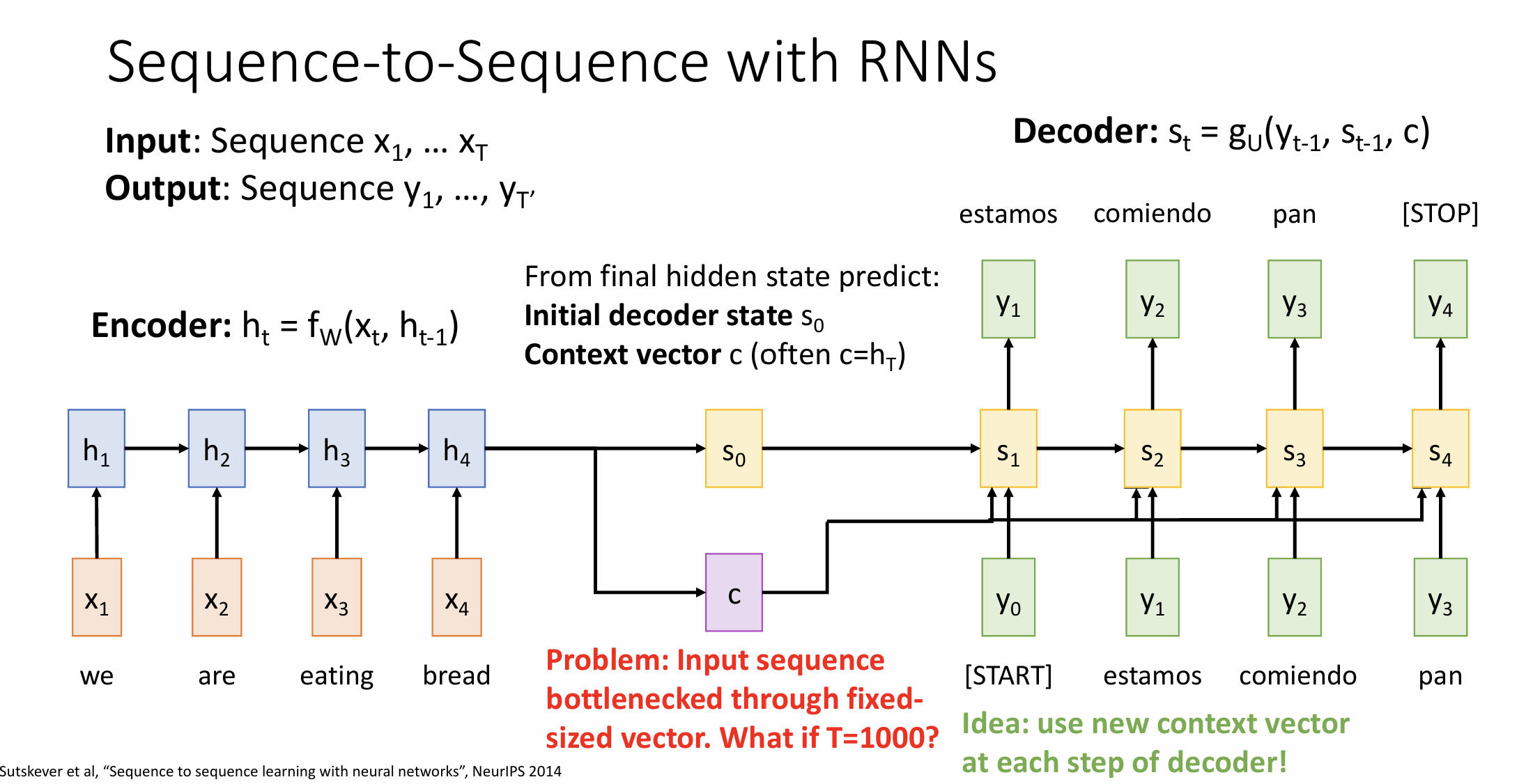
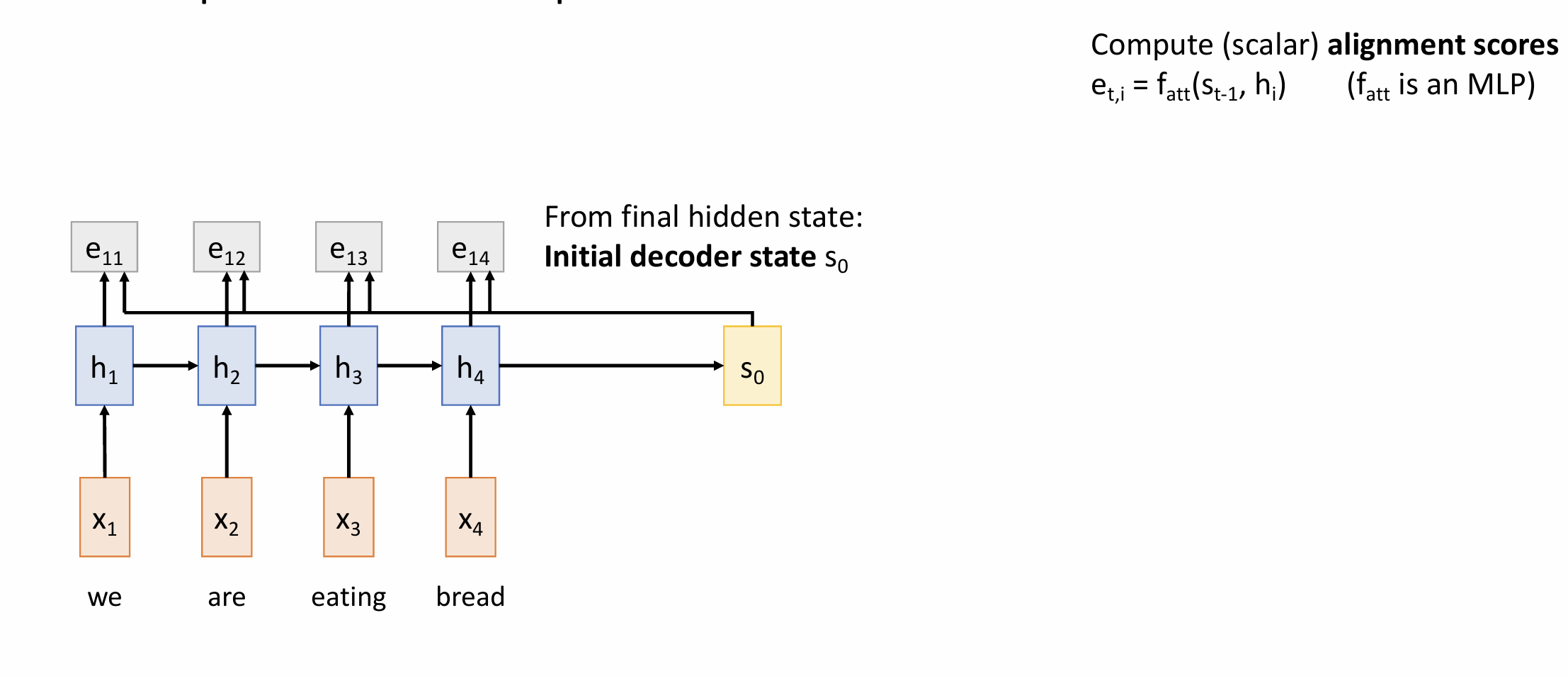
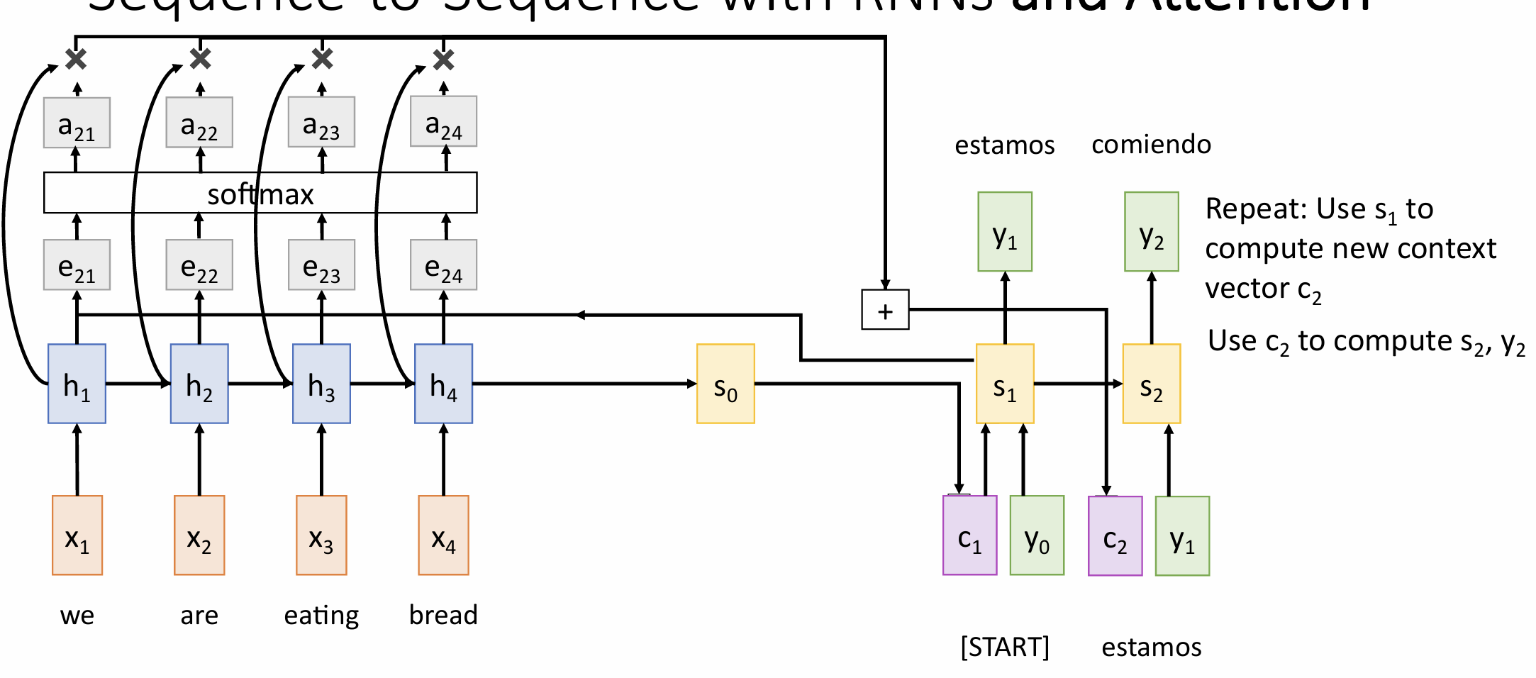
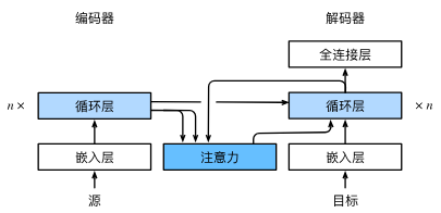
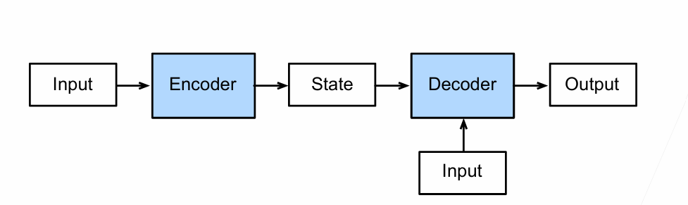
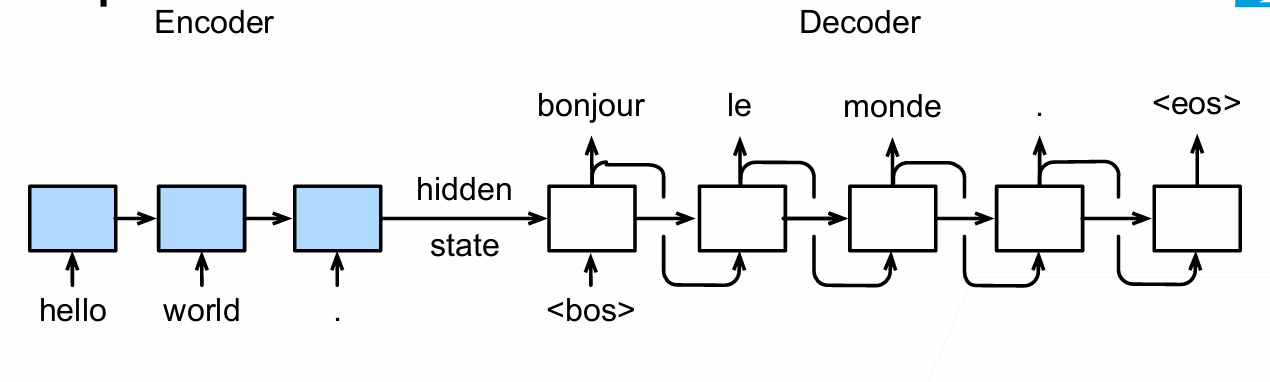
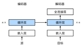
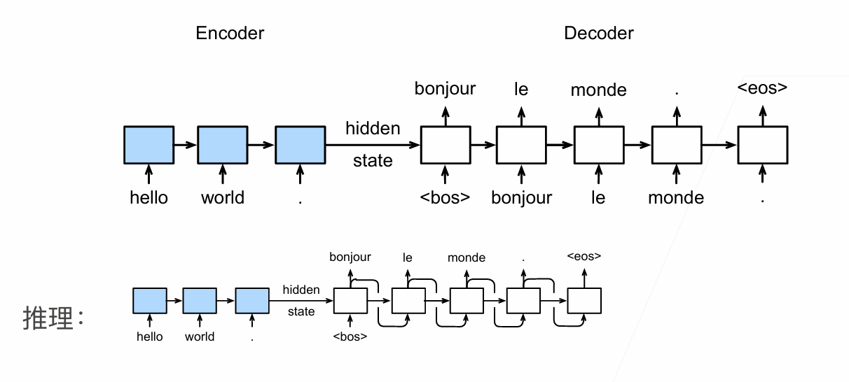
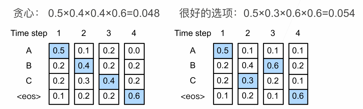
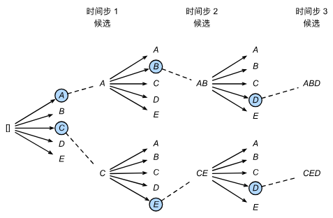
Sequence-to-Sequence with RNNs and Attention
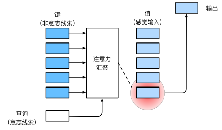
how much should we attend to each hidden state of the encoder given the current state of the decoder
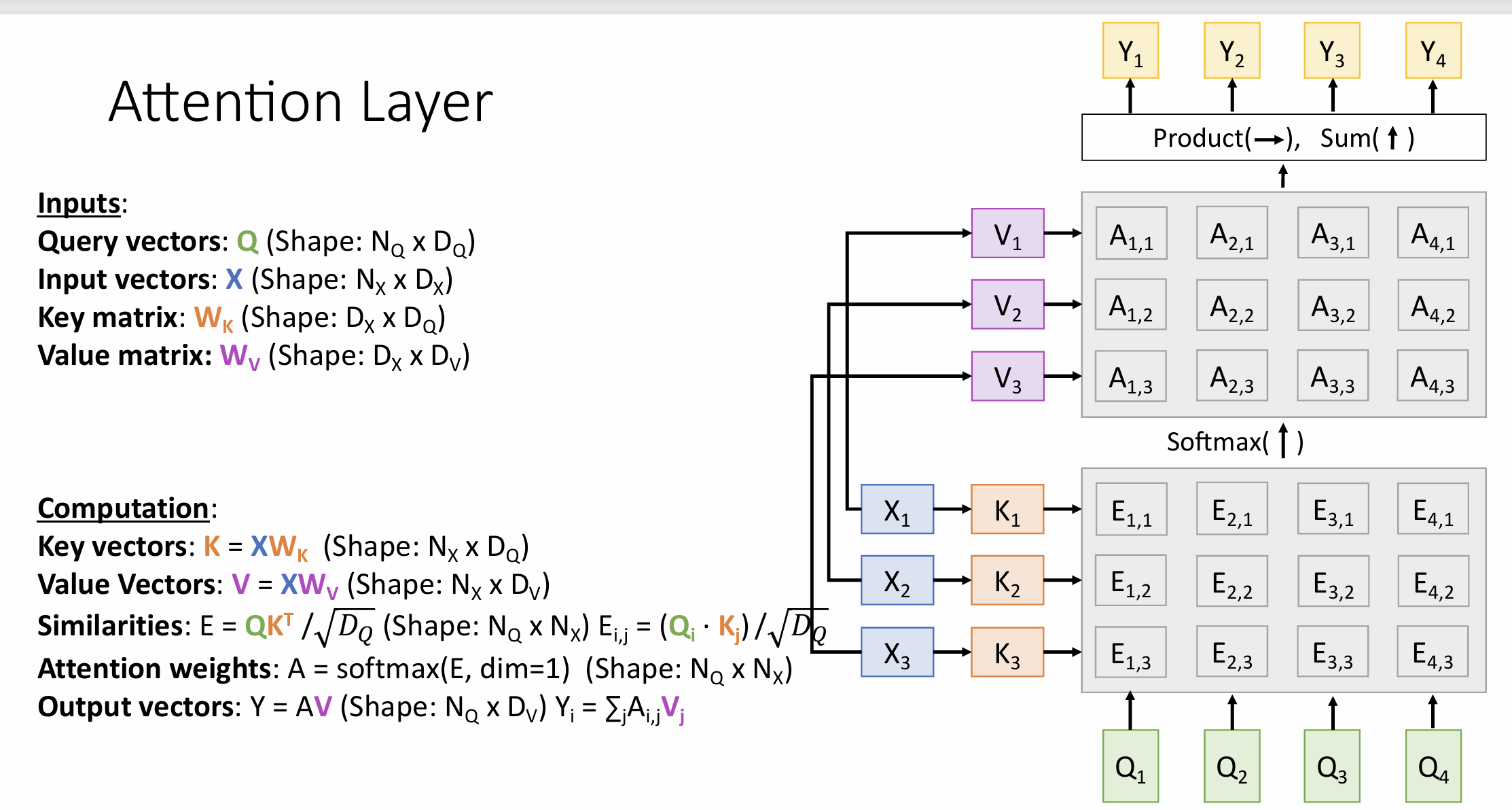
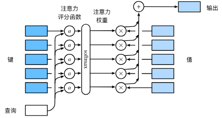
Attention Layer
scaled similarity function:dot product
multiple query vectors
seperate key and value
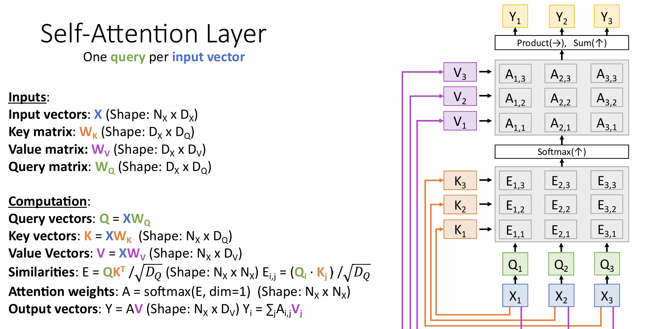
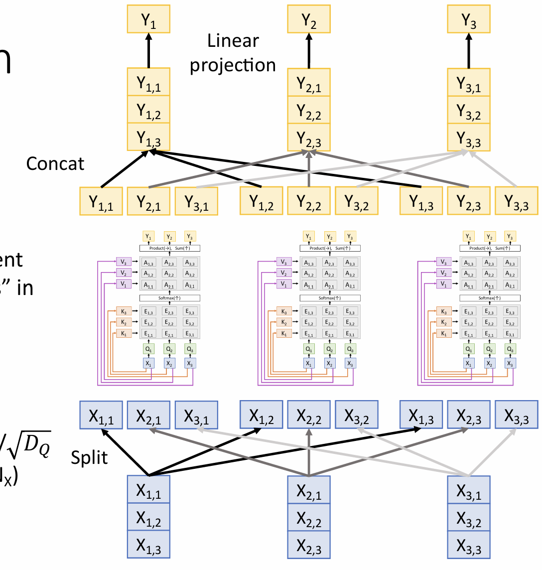
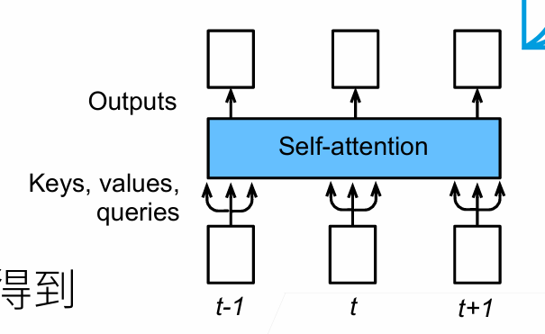
Self-Attention Layer
don’t know the order of the vectors->positon embedding
Y1:This produces the output of the self-attention layer at this position
Clearly the word at this position will have the highest softmax score, but sometimes it’s useful to attend to another word that is relevant to the current word.
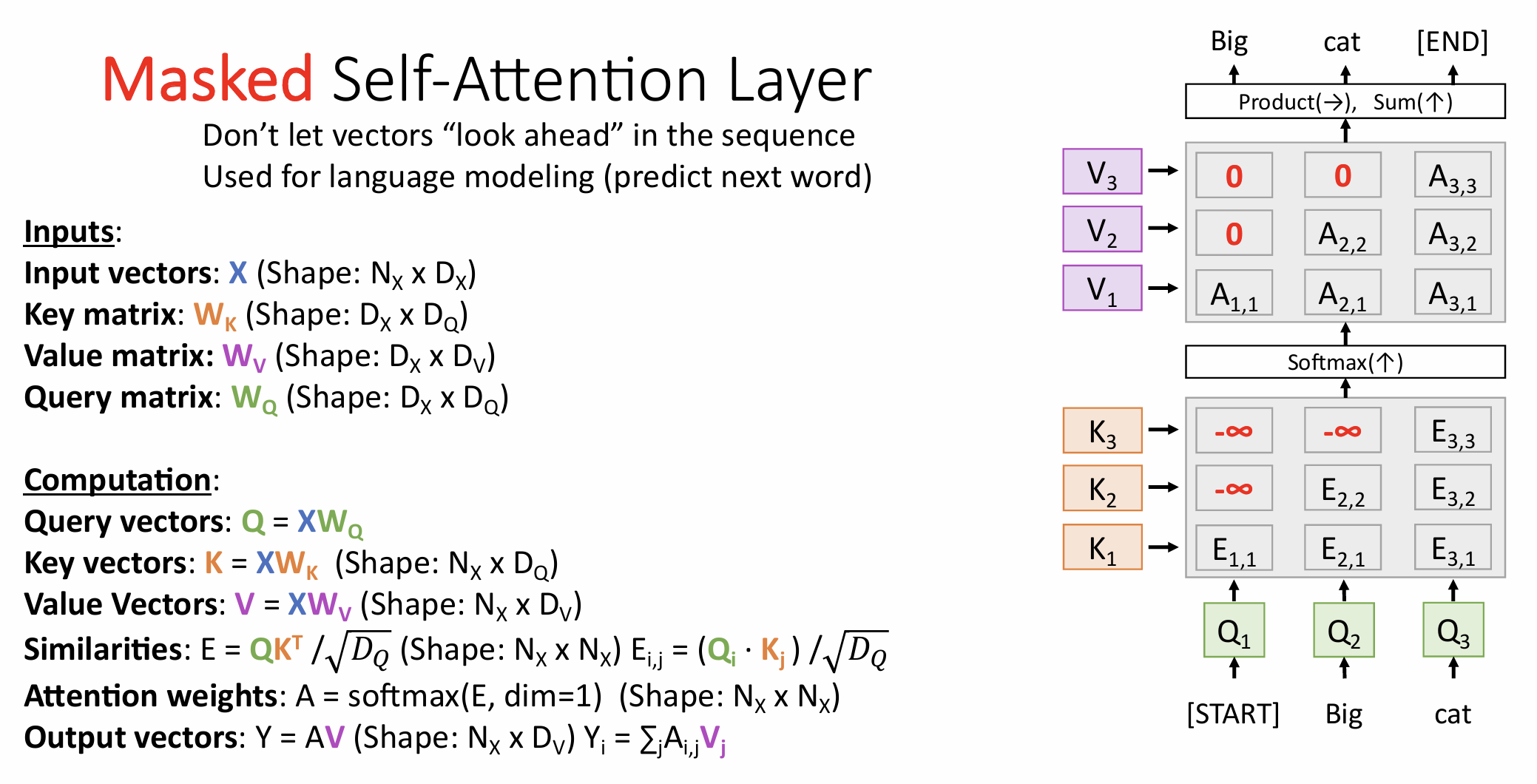
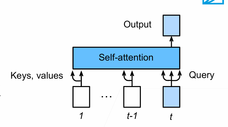
Masked Self-Attention Layer
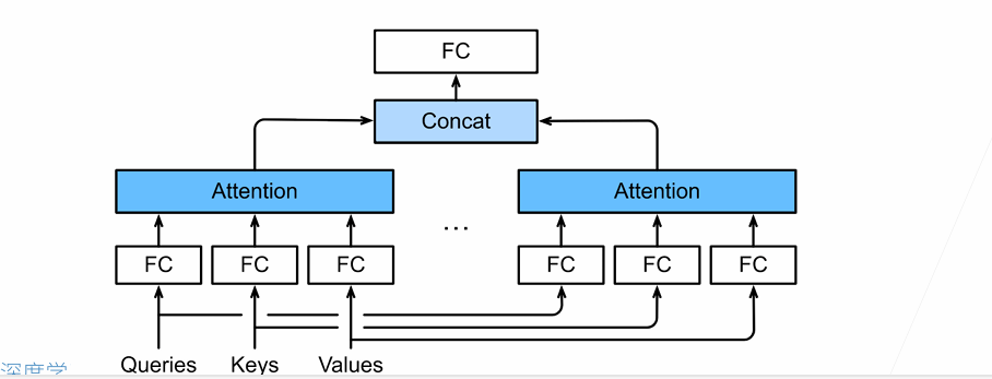
Multihead Self-Attention Layer
1.It expands the model’s ability to focus on different positions.
2.It gives the attention layer multiple “representation subspaces”.
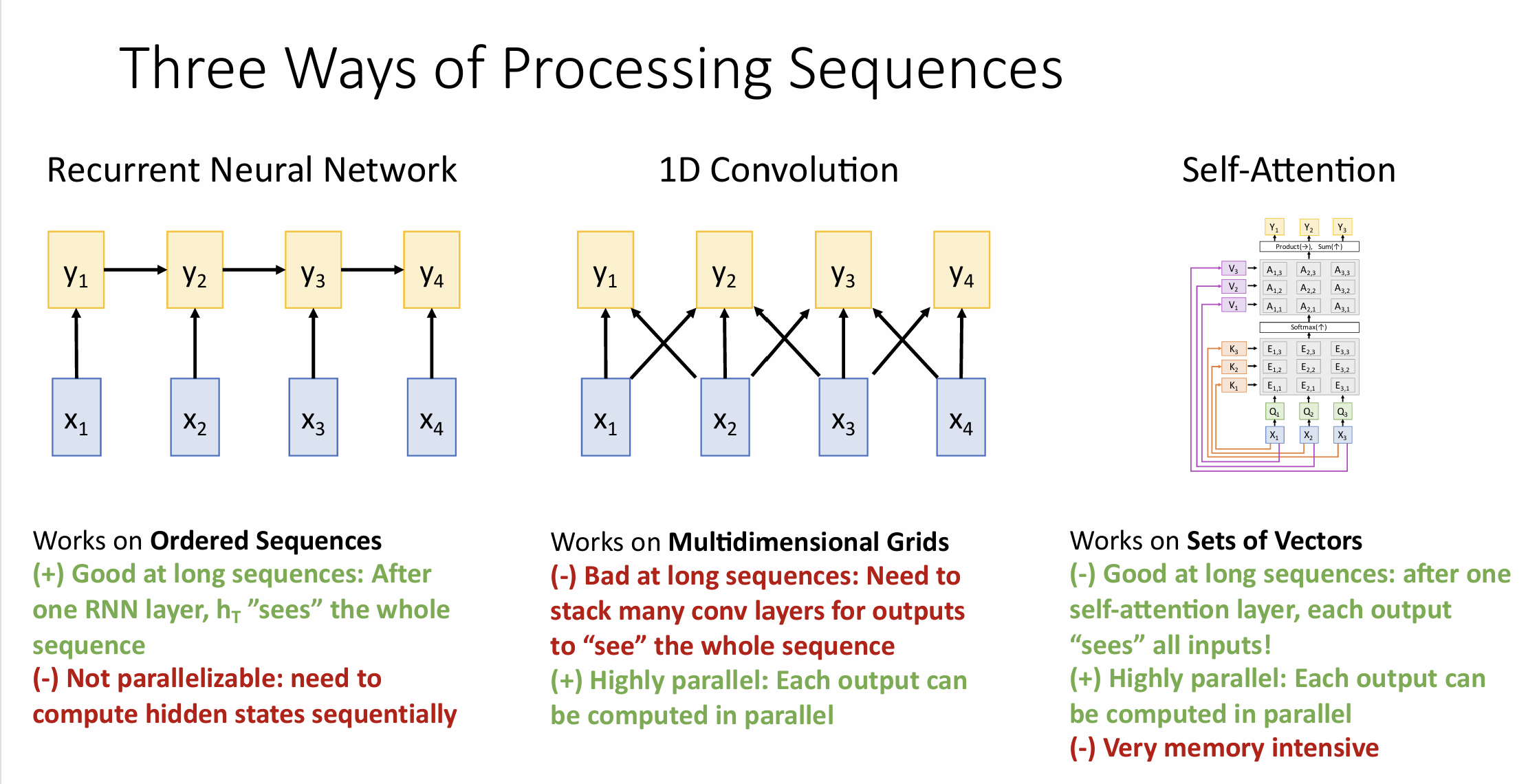
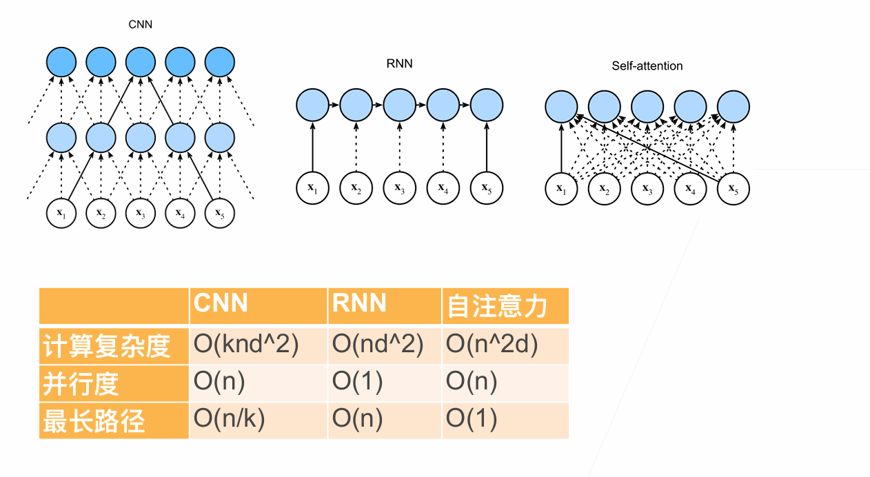
Three Ways of Processing Sequences
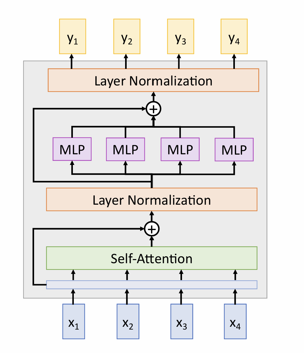
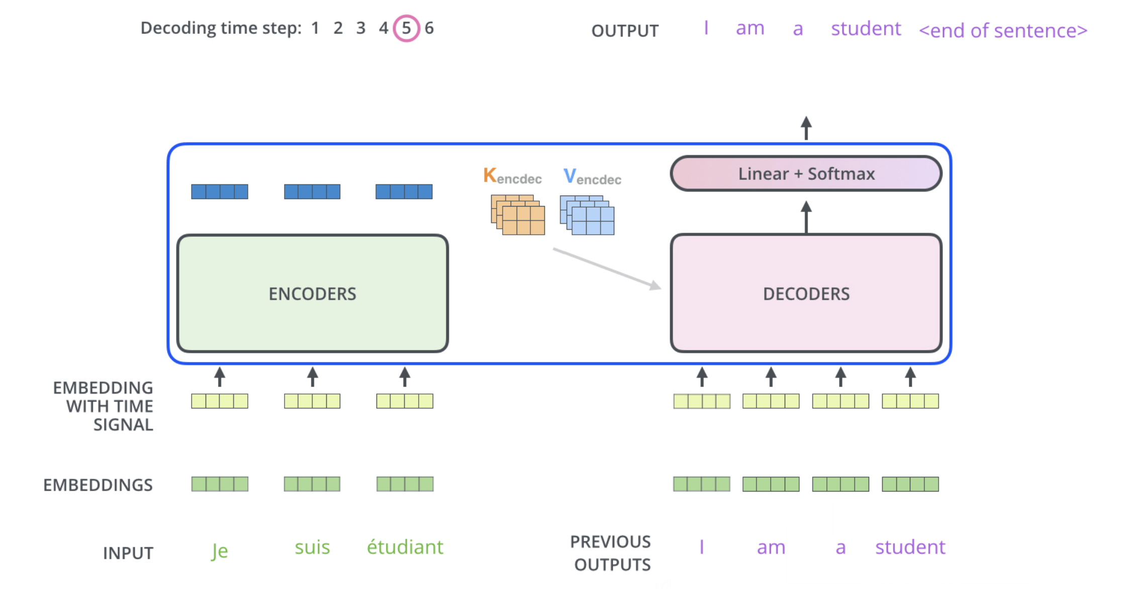
Transformer
For RNNs, instead of only encoding the whole sentence in a hidden state, each word has a corresponding hidden state that is passed all the way to the decoding stage. Then, the hidden states are used at each step of the RNN to decode.
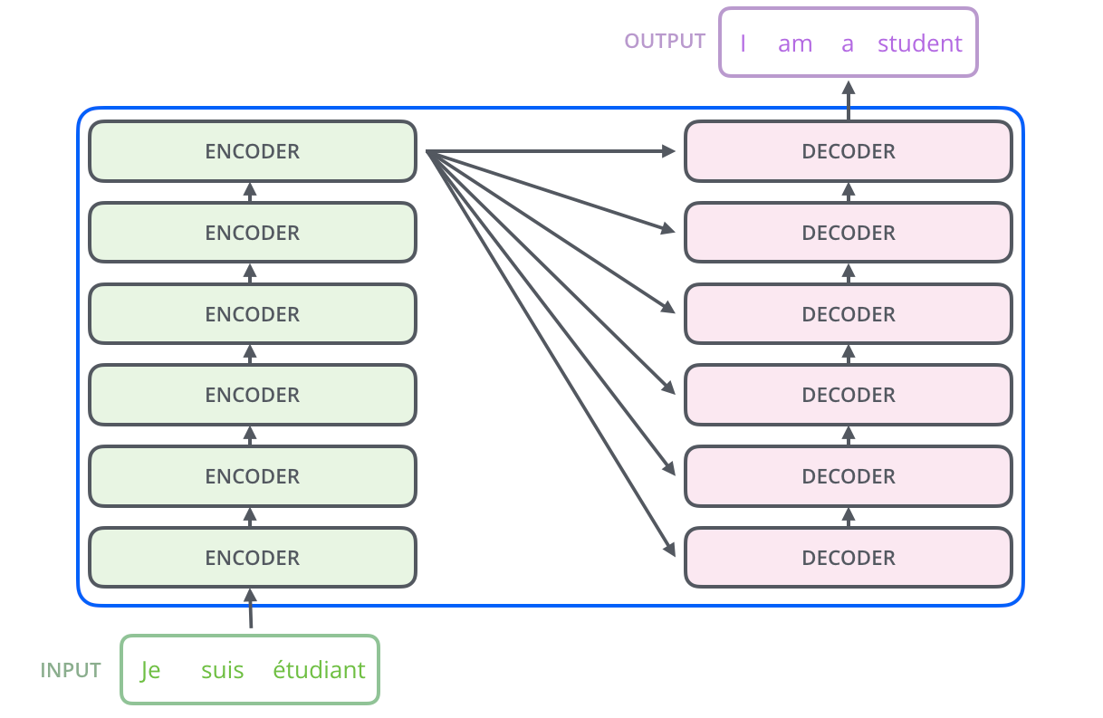
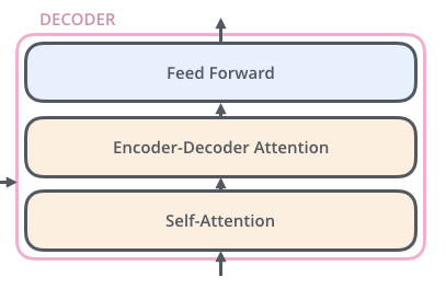
The Decoder Side
The encoder start by processing the input sequence. The output of the top encoder is then transformed into a set of attention vectors K and V. These are to be used by each decoder in its “encoder-decoder attention” layer which helps the decoder focus on appropriate places in the input sequence
Lecture 14: Visualizing and Understanding
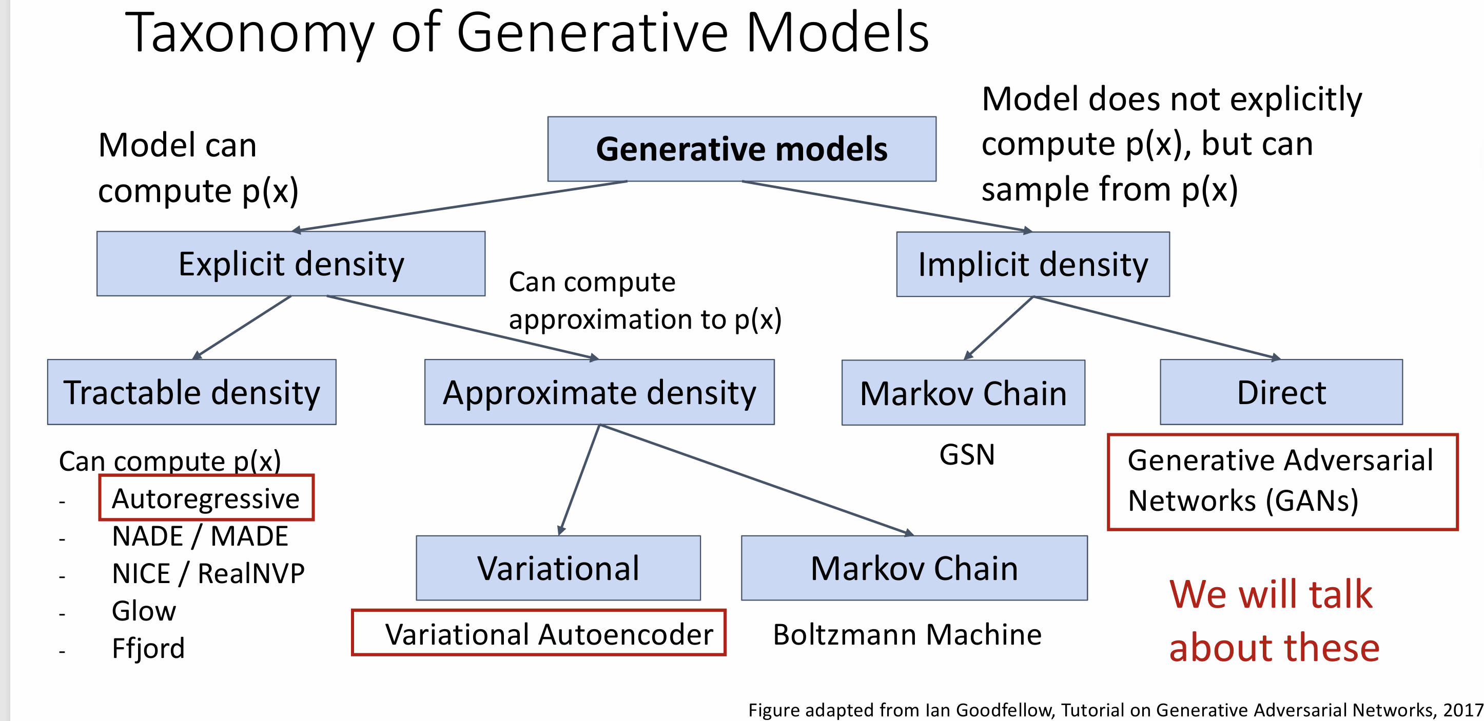
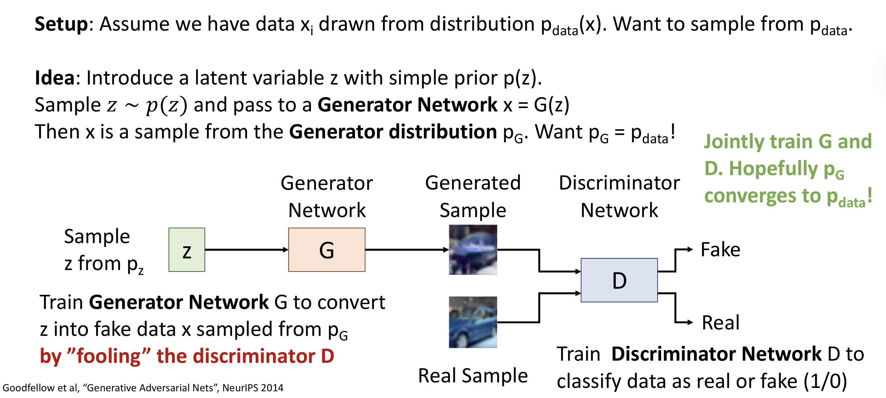
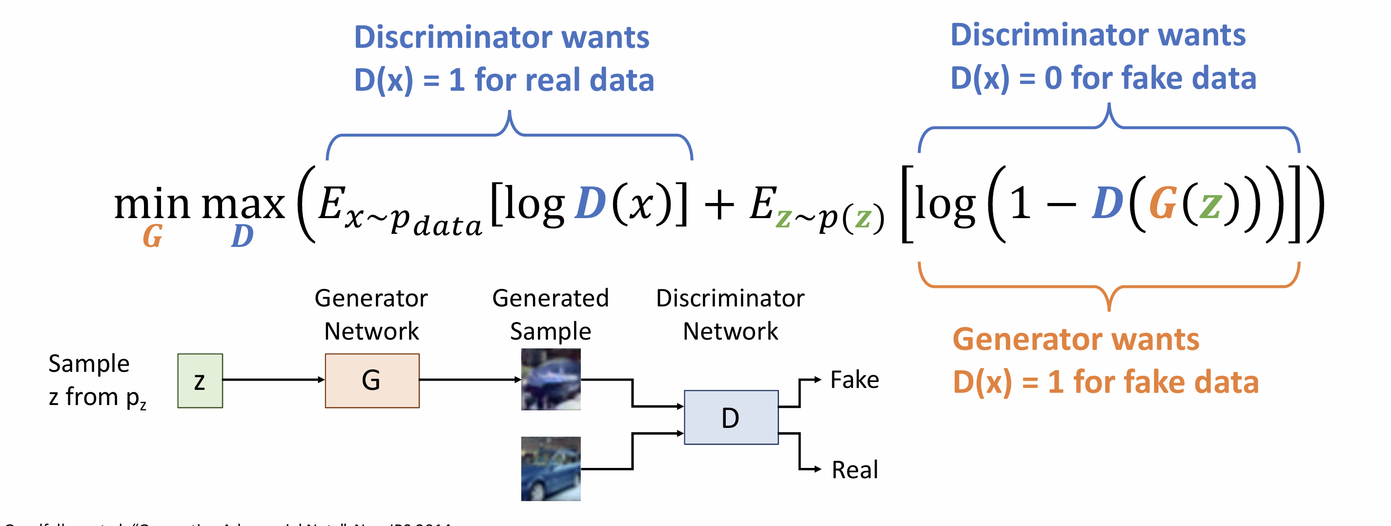
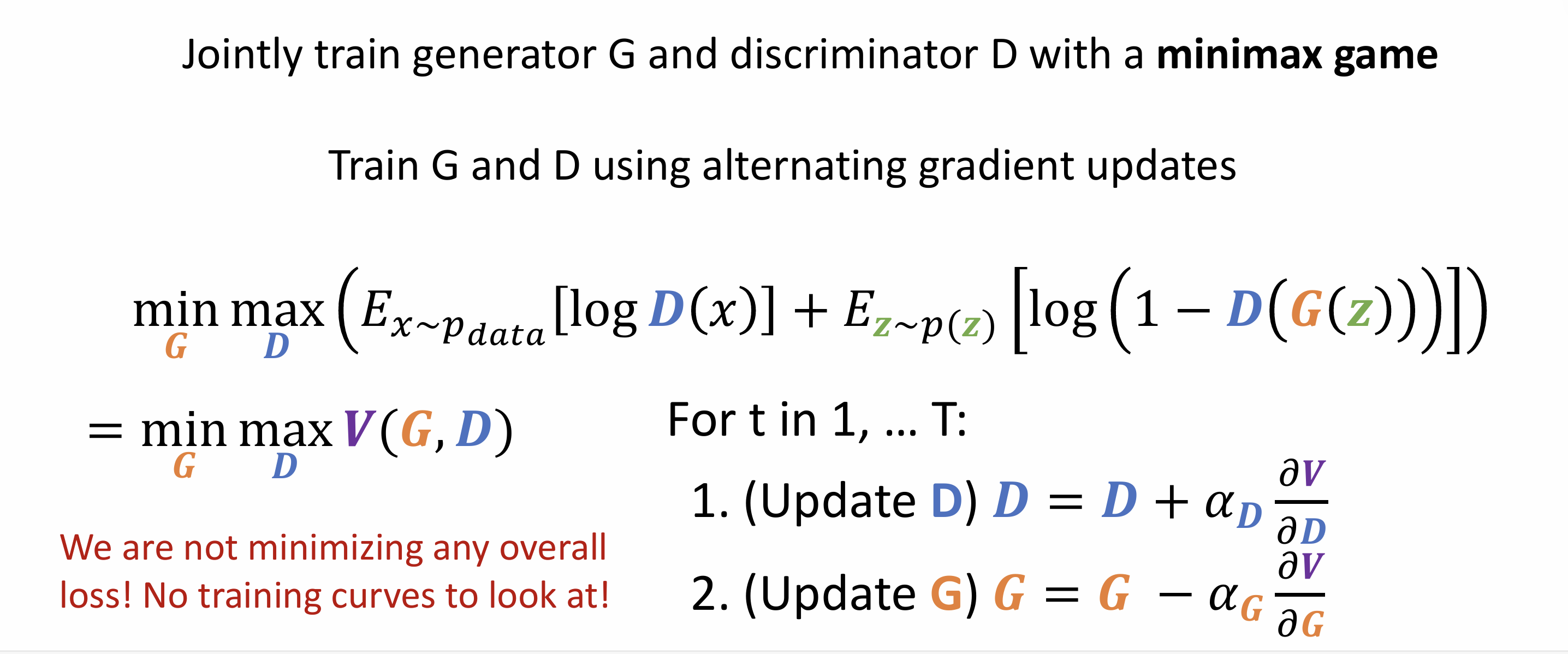
Lecture 19: Generative Models I
Discriminative Model: learn a probability distribution p(y|x)
Generative Model: learn a probability distribution p(x)
Conditional Generative Model: learn p(x|y)
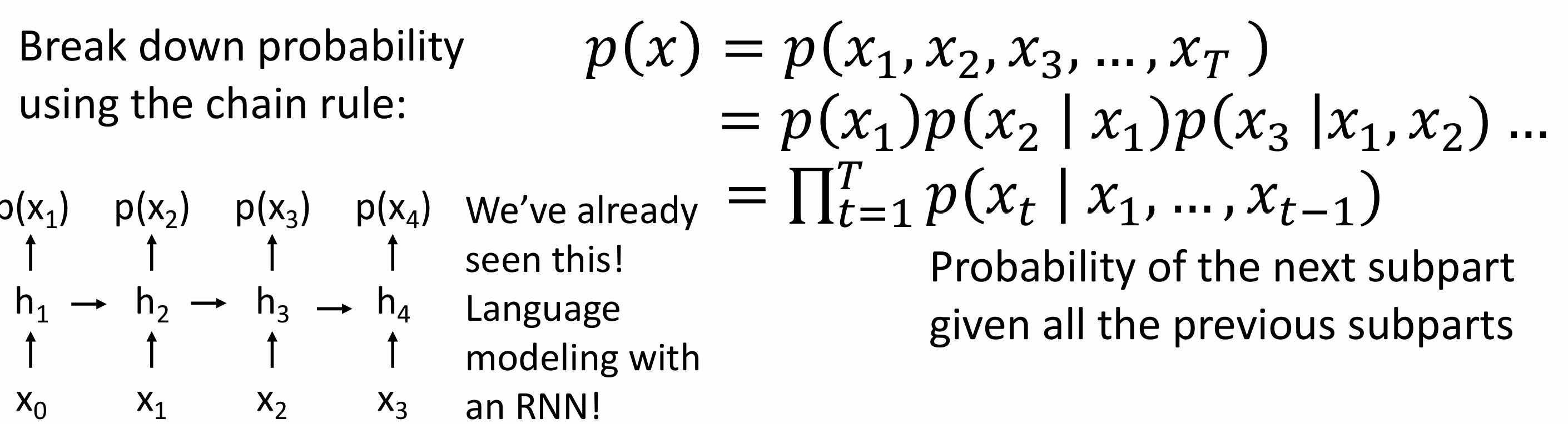
Autoregressive Models
goal:write down an explicit function for p(x)=f(x,W)
given dataset $x^{(i)}$,train the model by solving$W^*=argmax\prod_ip(x^{(i)})=argmax\sum_ilogf(x^{(i)},W)$
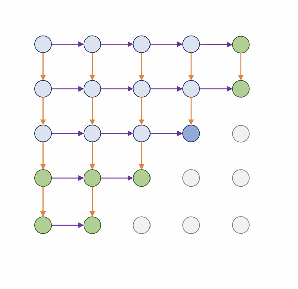
PixelRNN
generate from the upper left corner
compute a hidden state for each pixel that depends on hidden states and RGB values from the left and the above (LSTM)
$h{x,y}=f(h{x-1,y},h_{x,y-1},W)$
at each pixel,predict R,G,B:softmax over (0,1…255)
slow
PixelCNN
slow
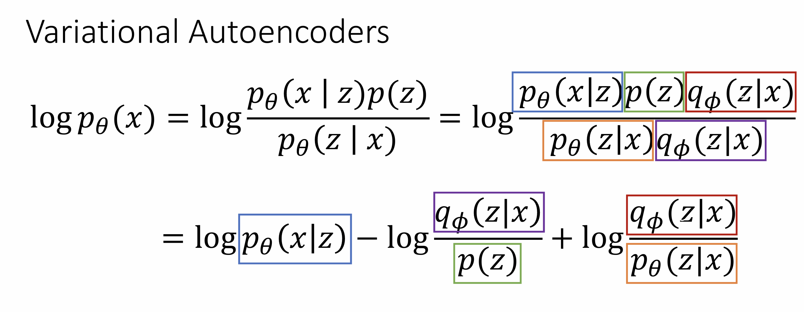
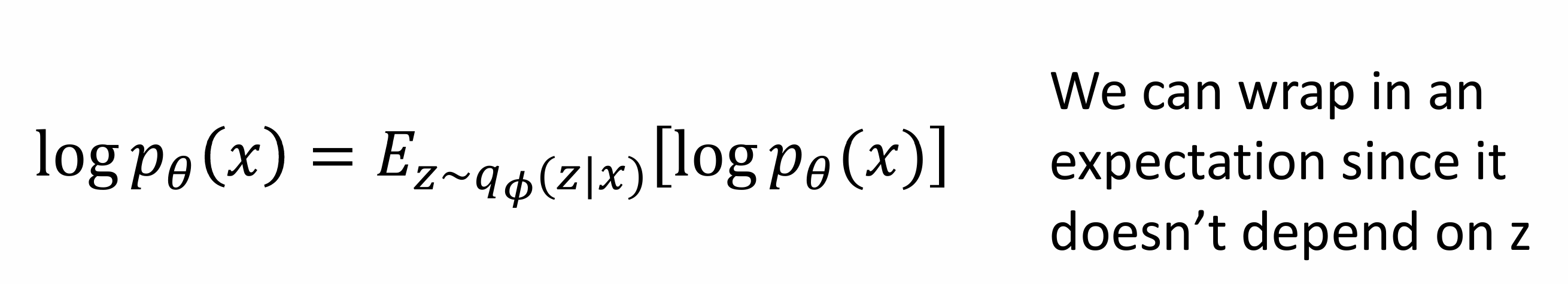
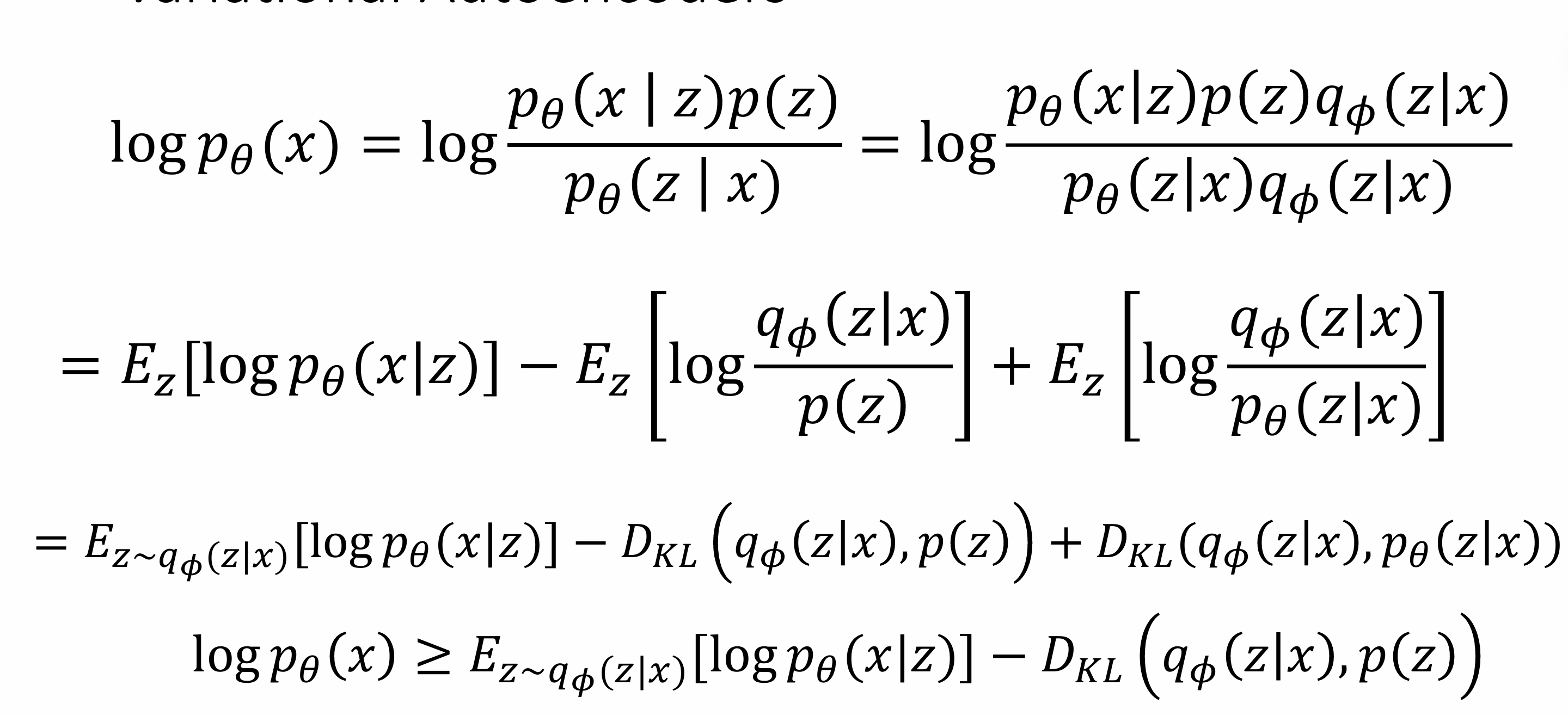
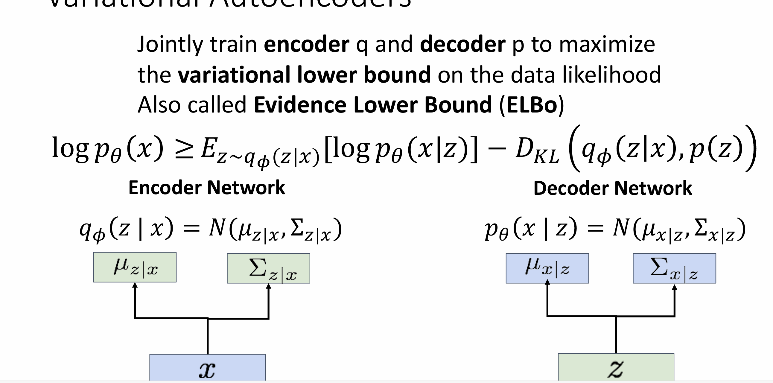
Variational Autoencoders
VAE define an intratable density that we cannot explicitly compute or optimize ,but can directly optimize a lower bound on the density
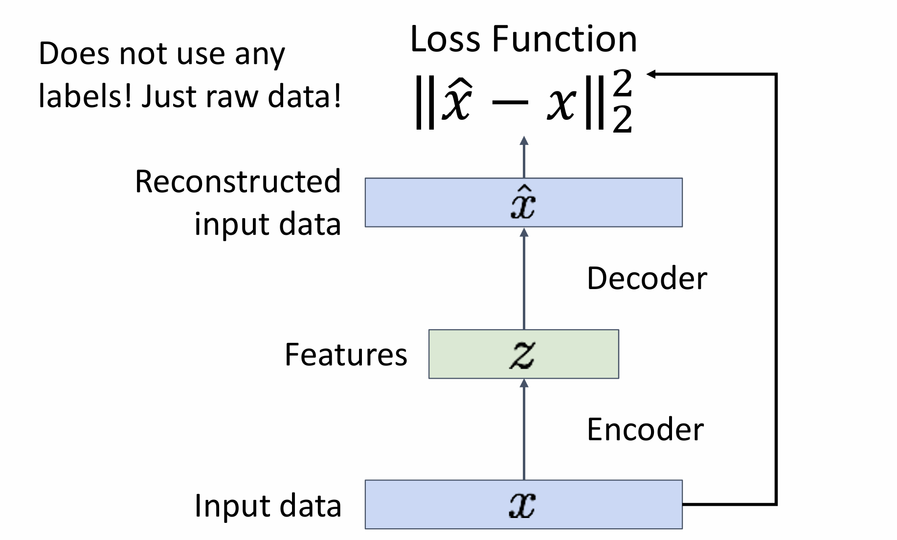
Autoencoders
cmompress to low dimention
cnn;up cnn
no probabilistic: no way to sample new data from learned model
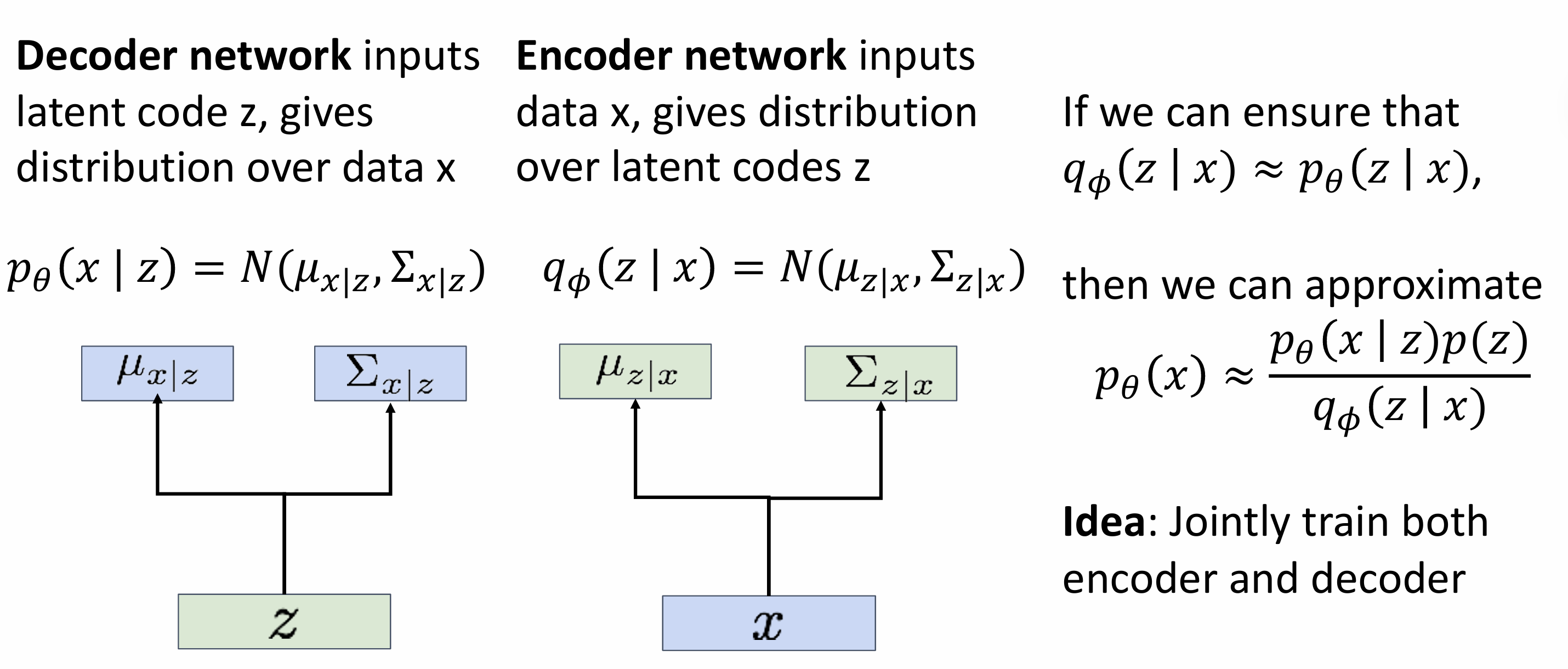
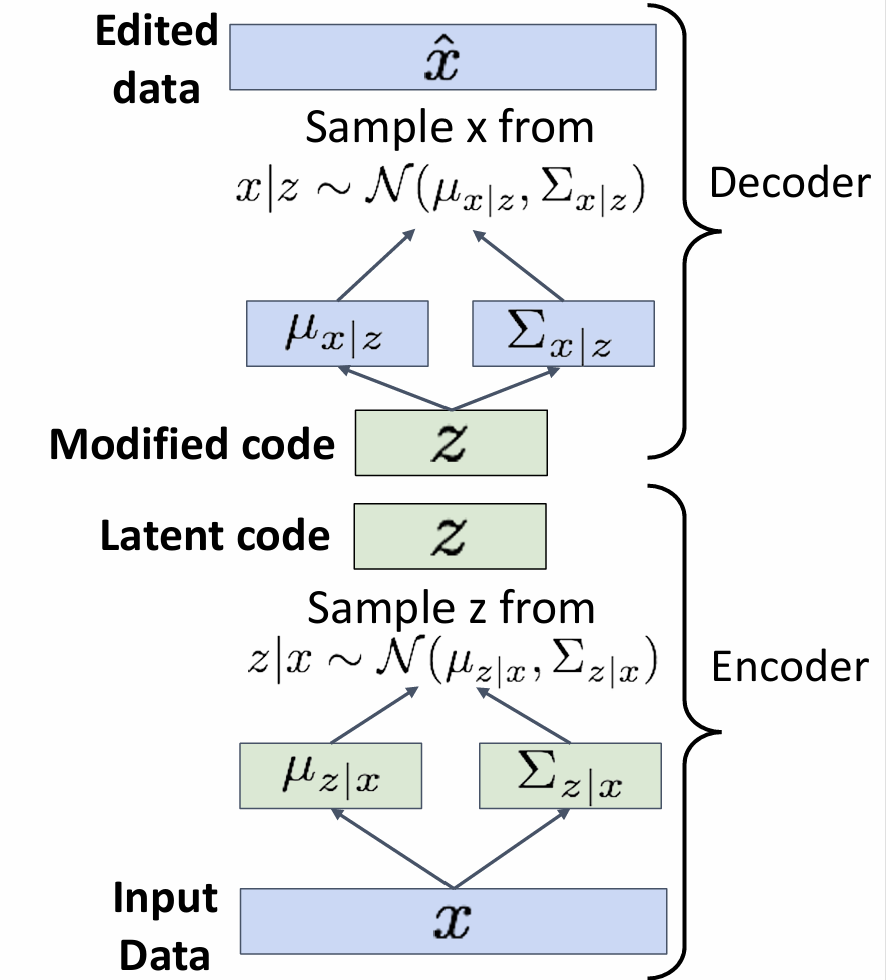
Variational Autoencoders
x is an image, z is latent factors(unobserved) used to generate x
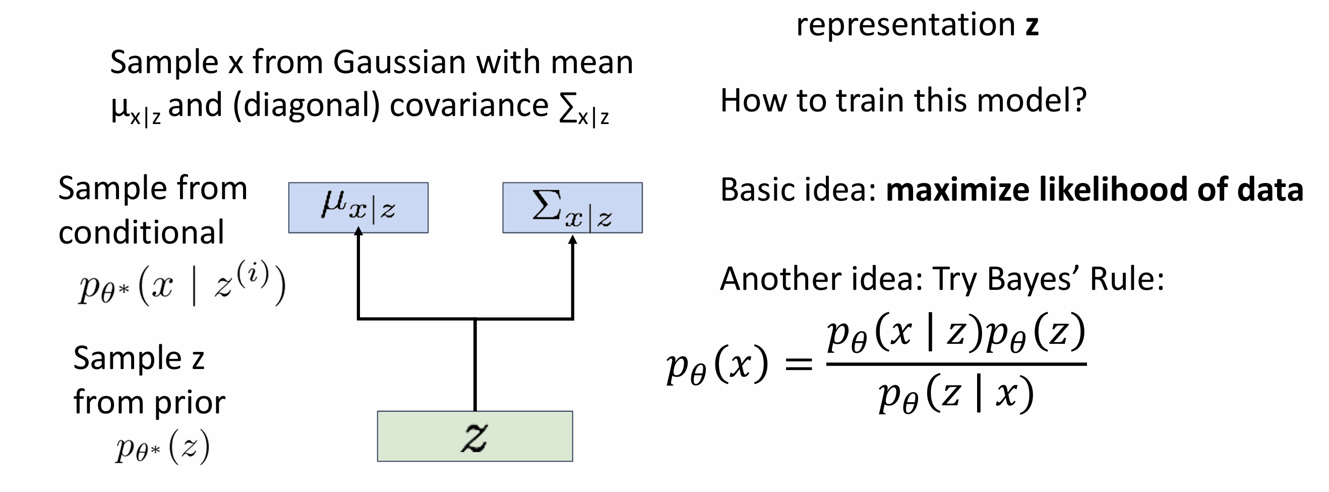
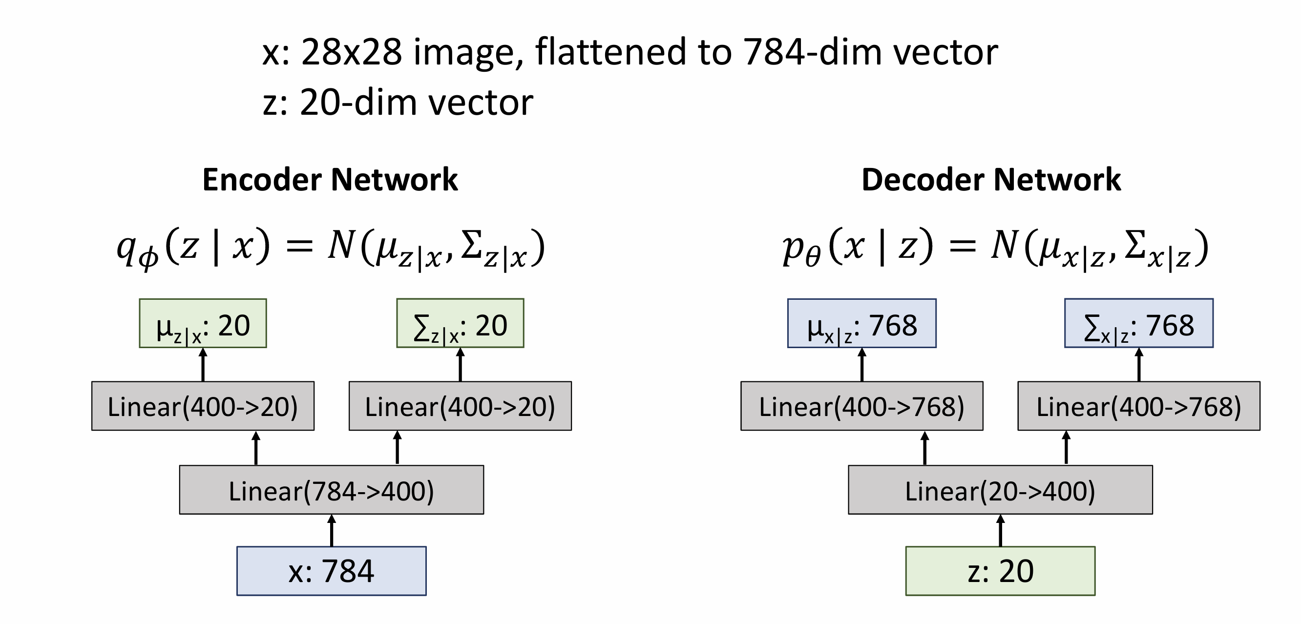
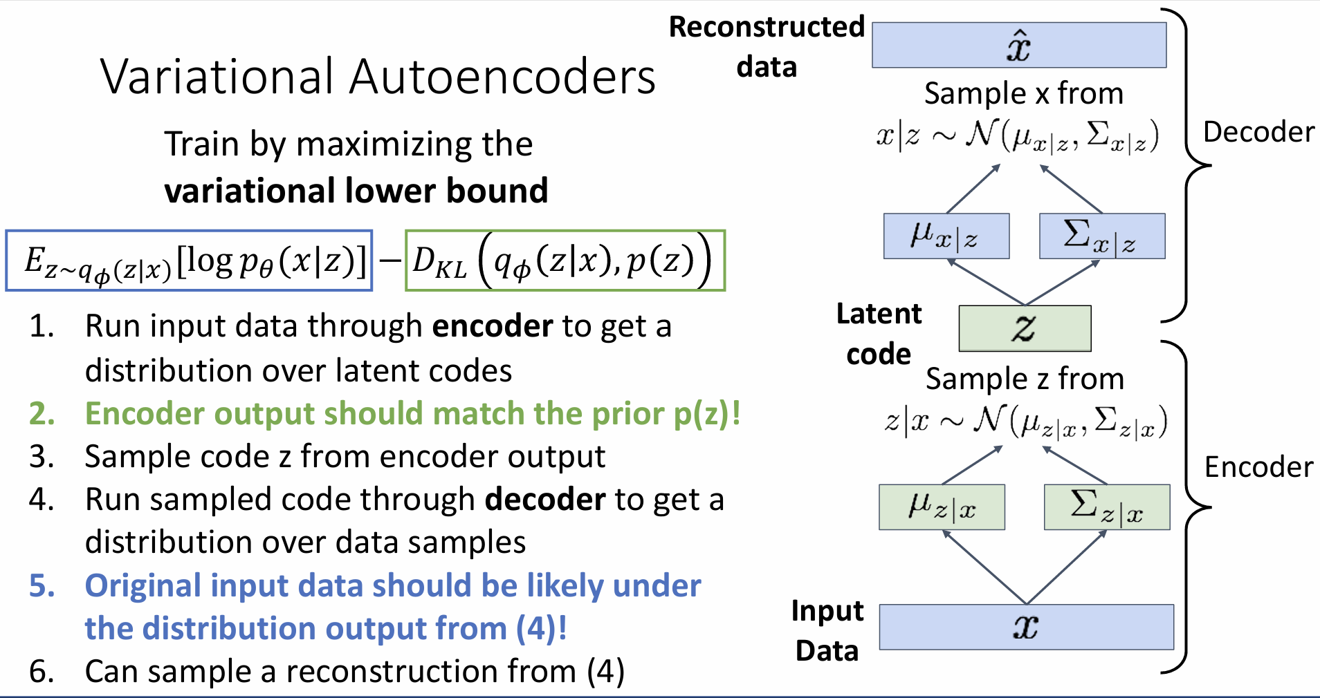
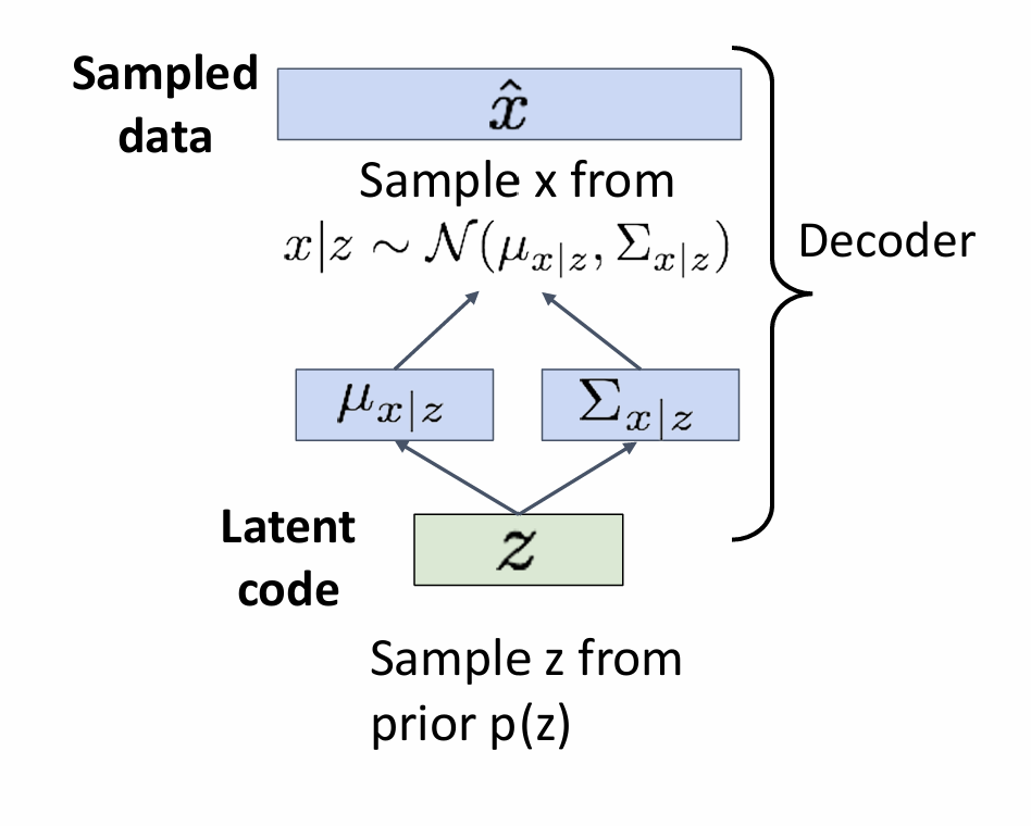
Decoder must be probabilistic: Decoder inputs z, outputs mean μx|z and (diagonal) covariance ∑x|z ->Sample x from Gaussian with mean μx|z and (diagonal) covariance ∑x|z
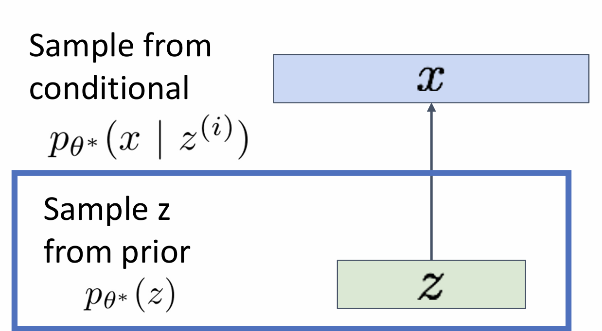
After training(test)
1.sample a new latent variable from the prior distribution
2.z-decoder-x’s distribution
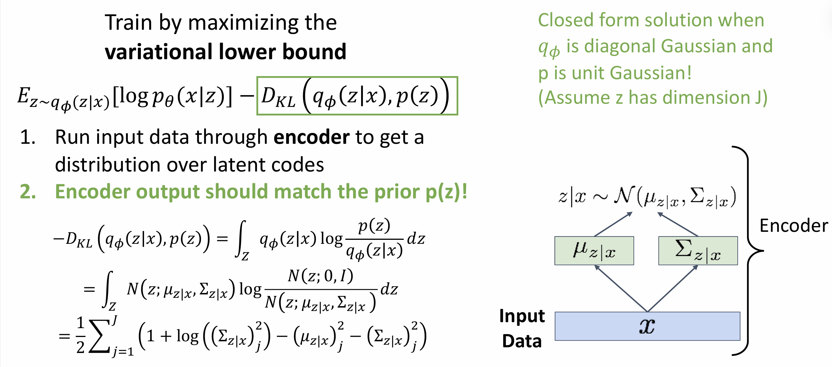
assume simple prior p(z): Gaussian
assume the probability over the image:gaussian with a number of the gaussian equal to the numer of pixels->parametrize:mean value and standard deviation value for each pixel
output a high dimentional gaussian distribution
represent p(x|z) with a neural network
Train
maximize likelihood
$p_{\theta}(x|z)$:decoder
$p_{\theta}(z)$:gaussian
Solution: Train another network (encoder) that learns $q{\phi}(z|x)=p{\theta}(z|x)$
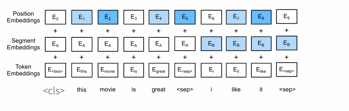
defforward(self, tokens, segments, valid_lens): X = self.token_embedding(tokens) + self.segment_embedding(segments) X = X + self.pos_embedding.data[:, :X.shape[1], :] for blk inself.blks: X = blk(X, valid_lens) return X
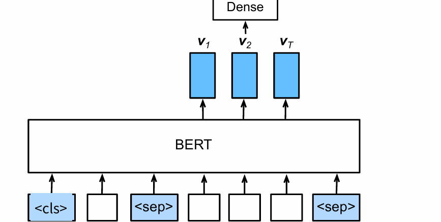
Masked Language Modeling
把要预测的位置的词所对应的encoder的输出拿到这里来预测位置的值
1 2 3 4 5 6 7 8 9 10 11 12 13 14 15 16 17 18 19
classMaskLM(nn.Module): """The masked language model task of BERT.""" def__init__(self, vocab_size, num_hiddens, num_inputs=768, **kwargs): super(MaskLM, self).__init__(**kwargs) self.mlp = nn.Sequential(nn.Linear(num_inputs, num_hiddens), nn.ReLU(), nn.LayerNorm(num_hiddens), nn.Linear(num_hiddens, vocab_size))
import collections import re from d2l import torch as d2l
将数据集读取到由文本行组成的列表中
1 2 3 4 5 6 7 8 9 10 11 12 13
d2l.DATA_HUB['time_machine'] = (d2l.DATA_URL + 'timemachine.txt', '090b5e7e70c295757f55df93cb0a180b9691891a') '''读取一本书''' defread_time_machine(): """Load the time machine dataset into a list of text lines.""" withopen(d2l.download('time_machine'), 'r') as f: lines = f.readlines() return [re.sub('[^A-Za-z]+', ' ', line).strip().lower() for line in lines] '''把不是字母和空格的都变成空格''' lines = read_time_machine() print(f' print(lines[0]) print(lines[10])
text lines: 3221 the time machine by h g wells twinkled and his usually pale face was flushed and animated the
每个文本序列被拆分成一个标记列表
文本行列表lines-文本序列line-词元列表tokens-词元token
1 2 3 4 5 6 7 8 9 10 11 12
deftokenize(lines, token='word'): """将文本行拆分为单词或字符标记。""" if token == 'word': return [line.split() for line in lines] elif token == 'char': return [list(line) for line in lines] else: print('错误:未知令牌类型:' + token)
tokens = tokenize(lines) for i inrange(11): print(tokens[i])
classVocab: """文本词表""" def__init__(self, tokens=None, min_freq=0, reserved_tokens=None): '''如果某个词出现次数小于min_freq,就不要了;保存那些被保留的词元, 例如:填充词元(“<pad>”); 序列开始词元(“<bos>”); 序列结束词元(“<eos>”)''' if tokens isNone: tokens = [] if reserved_tokens isNone: reserved_tokens = [] counter = count_corpus(tokens) self.token_freqs = sorted(counter.items(), key=lambda x: x[1], reverse=True)'''频率排序''' self.unk'''unknown记为0''', uniq_tokens = 0, ['<unk>'] + reserved_tokens uniq_tokens += [ token for token, freq inself.token_freqs if freq >= min_freq and token notin uniq_tokens] self.idx_to_token, self.token_to_idx = [], dict()'''下标和token相互转换''' for token in uniq_tokens: self.idx_to_token.append(token) self.token_to_idx[token] = len(self.idx_to_token) - 1
def__len__(self): returnlen(self.idx_to_token)
def__getitem__(self, tokens):'''token->index,返回index''' ifnotisinstance(tokens, (list, tuple)): returnself.token_to_idx.get(tokens, self.unk) return [self.__getitem__(token) for token in tokens]
defto_tokens(self, indices):'''index->token,返回token''' ifnotisinstance(indices, (list, tuple)): returnself.idx_to_token[indices] return [self.idx_to_token[index] for index in indices]
defcount_corpus(tokens): """统计标记的频率。""" iflen(tokens) == 0orisinstance(tokens[0], list): tokens = [token for line in tokens for token in line] return collections.Counter(tokens)
defload_corpus_time_machine(max_tokens=-1): """返回时光机器数据集的标记索引列表和词汇表。""" lines = read_time_machine() tokens = tokenize(lines, 'char') vocab = Vocab(tokens)'''对应字典''' corpus = [vocab[token] for line in tokens for token in line]'''每一个单词(这里是字母)的数字''' if max_tokens > 0: corpus = corpus[:max_tokens] return corpus, vocab
num_batches = num_subseqs // batch_size'''在n段里面取batch''' for i inrange(0, batch_size * num_batches, batch_size): initial_indices_per_batch = initial_indices[i:i + batch_size]'''取了batch size个开始的下标''' X = [data(j) for j in initial_indices_per_batch]'''生成batch size个段''' Y = [data(j + 1) for j in initial_indices_per_batch] yield torch.tensor(X), torch.tensor(Y)
num_hiddens = 512 net = RNNModelScratch(len(vocab), num_hiddens, d2l.try_gpu(), get_params, init_rnn_state, rnn) state = net.begin_state(X.shape[0], d2l.try_gpu()) Y, new_state = net(X.to(d2l.try_gpu()), state) Y.shape, len(new_state), new_state[0].shape
(torch.Size([10, 28]), 1, torch.Size([2, 512]))
首先定义预测函数来生成用户提供的prefix之后的新字符
1 2 3 4 5 6 7 8 9 10 11 12 13 14 15
defpredict_ch8(prefix, num_preds, net, vocab, device): """在`prefix`后面生成新字符。""" state = net.begin_state(batch_size=1, device=device) outputs = [vocab[prefix[0]]] get_input = lambda: torch.tensor([outputs[-1]], device=device).reshape( (1, 1)) for y in prefix[1:]: _, state = net(get_input(), state) outputs.append(vocab[y]) for _ inrange(num_preds): y, state = net(get_input(), state) outputs.append(int(y.argmax(dim=1).reshape(1))) return''.join([vocab.idx_to_token[i] for i in outputs])
defgrad_clipping(net, theta): """裁剪梯度。""" ifisinstance(net, nn.Module): params = [p for p in net.parameters() if p.requires_grad] else: params = net.params norm = torch.sqrt(sum(torch.sum((p.grad**2)) for p in params)) if norm > theta: for param in params: param.grad[:] *= theta / norm
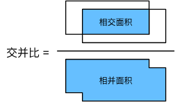
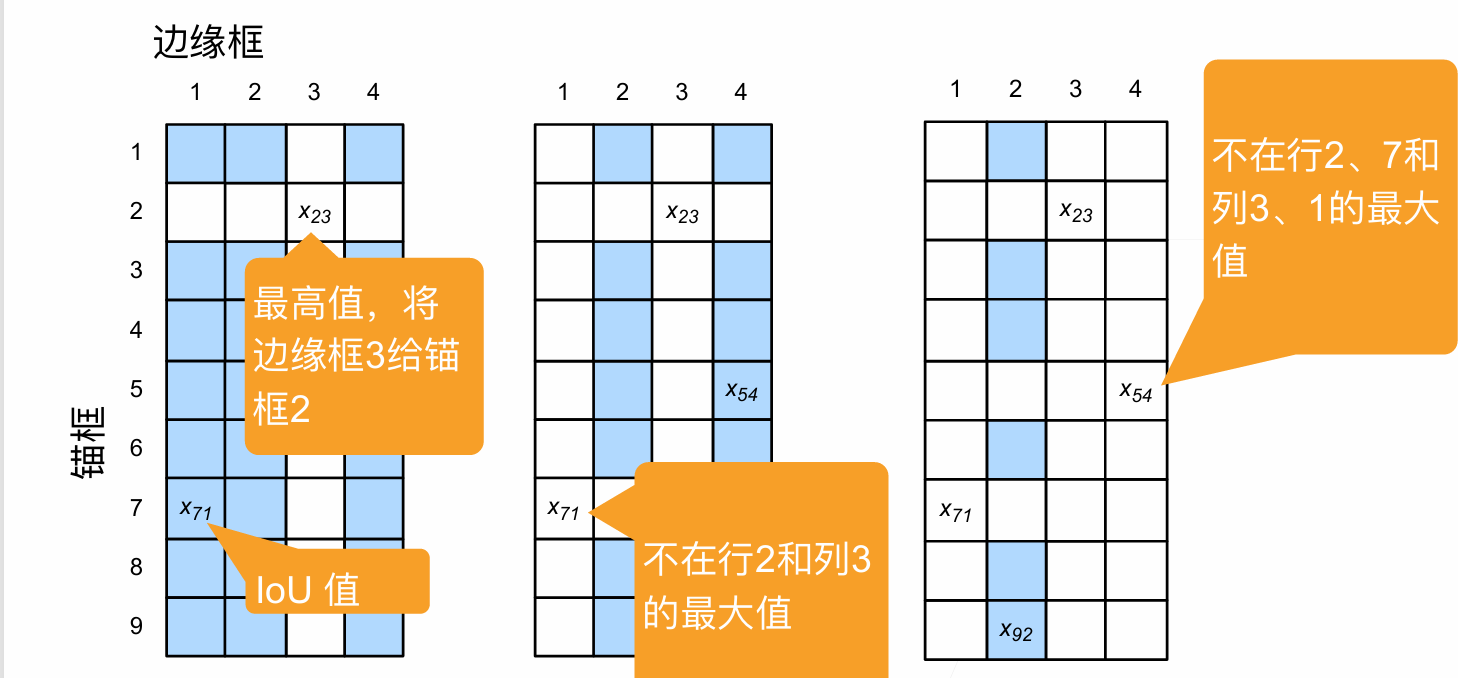
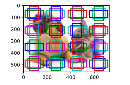
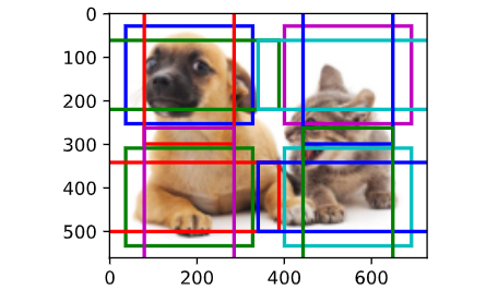
用ground truth 框(真实边界框)去标记所有1中生成的锚框(对应代码中的multibox_targe函数) 标记方法:计算所有锚框和ground-truth的IoU值,给每一个锚框分配一个真实边界框(小于阈值的为背景,大于的选一个最接近的ground-truth),即用最近的那个标记,详见3.